Transform data with T-SQL in a Fabric warehouse

A Microsoft Fabric warehouse provides full read-write T-SQL capabilities for transforming data. Unlike the SQL analytics endpoint on a lakehouse (which is read-only), a warehouse supports INSERT, UPDATE, DELETE, and CREATE TABLE AS SELECT (CTAS) statements. This makes the warehouse the right place for building transformation logic that needs to persist results.

In this exercise, you work with staging sales, customer, and product data in a Fabric warehouse. You write T-SQL queries to filter, join, and aggregate data. You create a view for reusable transformation logic, build a stored procedure with parameters for repeatable processing, and create and load dimensional tables. These tasks reinforce the query, view, stored procedure, and dimensional modeling techniques covered in this module.

This exercise takes approximately 45 minutes to complete.

Tip: For related training content, see Transform data using T-SQL in Microsoft Fabric.

Note: This exercise includes optional prompts to explore Copilot capabilities.

Set up the environment

Note: You need access to a Fabric paid or trial capacity to complete this exercise. For information about the free Fabric trial, see Fabric trial.

Create a workspace

In this task, you create a Fabric workspace for the exercise.

Navigate to the Microsoft Fabric home page at https://app.fabric.microsoft.com/home?experience=fabric in a browser, and sign in with your Fabric credentials.
In the menu bar on the left, select Workspaces (the icon looks similar to 🗇).
Create a new workspace with a name of your choice, selecting a licensing mode that includes Fabric capacity (Trial, Premium, or Fabric).
When your new workspace opens, it should be empty.

Create a warehouse

In this task, you create a warehouse to store and transform data.

On the menu bar on the left, select Create. In the New page, under the Data Warehouse section, select Warehouse. Give it a name of your choice.

Note: If the Create option is not pinned to the sidebar, select the ellipsis (…) option first.

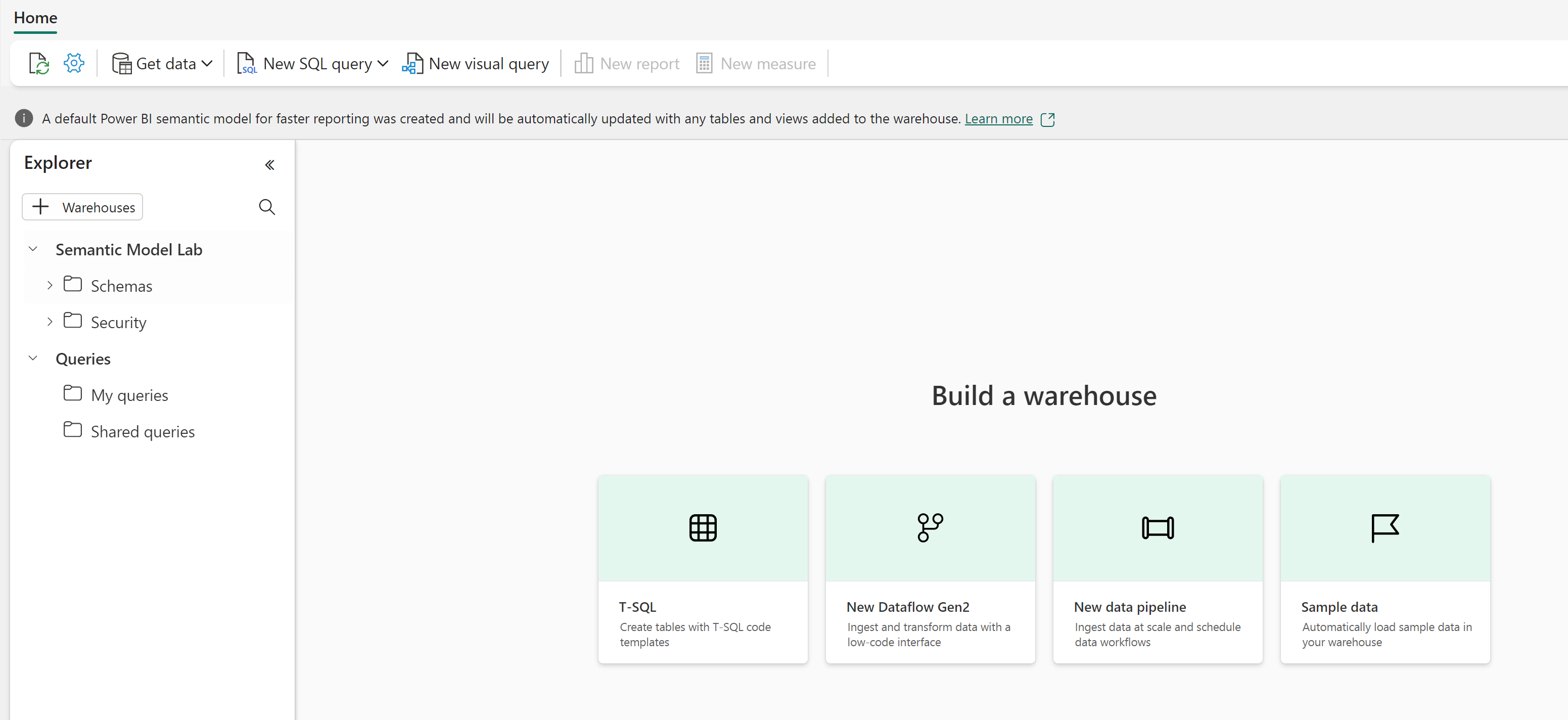
After a minute or so, a new warehouse is created.

Create staging tables and load sample data

In this task, you create schemas and staging tables, then insert sample data that simulates raw sales transactions, customers, and products.

In your warehouse, select New SQL query from the toolbar and run the following T-SQL to create schemas and staging tables:

Tip: If you are in a lab VM and have any problems entering the code, you can download the 26d-snippets.txt file from https://github.com/MicrosoftLearning/mslearn-fabric/raw/main/Allfiles/Labs/26d/26d-snippets.txt, saving it on the VM. The file contains all the T-SQL code used in this lab.

 -- Create schemas for organizing objects
 CREATE SCHEMA staging;
 GO
 CREATE SCHEMA dim;
 GO
 CREATE SCHEMA fact;
 GO
 CREATE SCHEMA gold;
 GO

 -- Staging: Customers
 CREATE TABLE staging.customers (
     customer_id VARCHAR(20) NOT NULL,
     customer_name VARCHAR(100),
     segment VARCHAR(50),
     region VARCHAR(50)
 );

 INSERT INTO staging.customers VALUES
 ('C001', 'Contoso Ltd', 'Enterprise', 'East'),
 ('C002', 'Fabrikam Inc', 'SMB', 'West'),
 ('C003', 'Northwind Traders', 'Enterprise', 'North'),
 ('C004', 'Adventure Works', 'SMB', 'South'),
 ('C005', 'Woodgrove Bank', 'Enterprise', 'West');

 -- Staging: Products
 CREATE TABLE staging.products (
     product_id VARCHAR(20) NOT NULL,
     product_name VARCHAR(100),
     category VARCHAR(50),
     unit_price DECIMAL(10,2)
 );

 INSERT INTO staging.products VALUES
 ('P001', 'Widget Alpha', 'Widgets', 15.00),
 ('P002', 'Widget Beta', 'Widgets', 22.50),
 ('P003', 'Gadget Gamma', 'Gadgets', 45.00),
 ('P004', 'Gadget Delta', 'Gadgets', 60.00),
 ('P005', 'Component Epsilon', 'Components', 9.99);

 -- Staging: Orders
 CREATE TABLE staging.orders (
     order_id INT NOT NULL,
     customer_id VARCHAR(20),
     product_id VARCHAR(20),
     order_date DATE,
     quantity INT,
     unit_price DECIMAL(10,2),
     discount DECIMAL(10,2),
     status VARCHAR(20)
 );

 INSERT INTO staging.orders VALUES
 (1, 'C001', 'P001', '2026-01-15', 10, 15.00, NULL, 'Completed'),
 (2, 'C001', 'P003', '2026-01-22', 5, 45.00, 10.00, 'Completed'),
 (3, 'C002', 'P002', '2026-02-10', 20, 22.50, NULL, 'Completed'),
 (4, 'C003', 'P004', '2026-02-18', 3, 60.00, 5.00, 'Completed'),
 (5, 'C002', 'P001', '2026-03-05', 15, 15.00, NULL, 'Completed'),
 (6, 'C004', 'P003', '2026-03-12', 8, 45.00, NULL, 'Pending'),
 (7, 'C001', 'P002', '2026-04-01', 12, 22.50, NULL, 'Completed'),
 (8, 'C003', 'P001', '2026-04-15', 25, 15.00, 2.50, 'Completed'),
 (9, 'C005', 'P004', '2026-05-02', 6, 60.00, NULL, 'Completed'),
 (10, 'C002', 'P005', '2026-05-20', 40, 9.99, NULL, 'Completed'),
 (11, 'C005', 'P002', '2026-06-08', 14, 22.50, 5.00, 'Completed'),
 (12, 'C003', 'P003', '2026-06-15', 2, 45.00, NULL, 'Completed');

 -- Staging: Dates (for the date dimension)
 CREATE TABLE staging.dates (
     calendar_date DATE NOT NULL,
     calendar_year INT,
     calendar_month INT,
     month_name VARCHAR(20),
     calendar_quarter INT
 );

 INSERT INTO staging.dates VALUES
 ('2026-01-15', 2026, 1, 'January', 1),
 ('2026-01-22', 2026, 1, 'January', 1),
 ('2026-02-10', 2026, 2, 'February', 1),
 ('2026-02-18', 2026, 2, 'February', 1),
 ('2026-03-05', 2026, 3, 'March', 1),
 ('2026-03-12', 2026, 3, 'March', 1),
 ('2026-04-01', 2026, 4, 'April', 2),
 ('2026-04-15', 2026, 4, 'April', 2),
 ('2026-05-02', 2026, 5, 'May', 2),
 ('2026-05-20', 2026, 5, 'May', 2),
 ('2026-06-08', 2026, 6, 'June', 2),
 ('2026-06-15', 2026, 6, 'June', 2);

Use the Refresh button in the Explorer pane to verify the tables appear under the staging schema.

Transform data with T-SQL queries

Querying is the first step in any data transformation workflow. In this section, you write T-SQL queries that filter, shape, join, aggregate, and apply window functions to the staging data.

Select New SQL query to open a new query tab. Run the following query to filter completed orders and add calculated columns:

 -- Filter completed orders and add calculated columns
 SELECT
     order_id,
     customer_id,
     order_date,
     quantity,
     unit_price,
     quantity * unit_price AS line_total,
     ISNULL(discount, 0) AS discount,
     (quantity * unit_price) - ISNULL(discount, 0) AS net_amount,
     CASE
         WHEN quantity * unit_price > 200 THEN 'High'
         WHEN quantity * unit_price > 100 THEN 'Medium'
         ELSE 'Standard'
     END AS order_tier
 FROM staging.orders
 WHERE status = 'Completed';

This query filters to completed orders, replaces null discounts with zero using ISNULL, calculates line totals and net amounts, and classifies each order into a tier using a CASE expression.

Select New SQL query and run the following query to join orders with customers and aggregate by region and segment:

 -- Join orders with customers and aggregate by region and segment
 SELECT
     c.region,
     c.segment,
     COUNT(*) AS order_count,
     SUM(o.quantity * o.unit_price) AS total_sales,
     AVG(o.quantity * o.unit_price) AS avg_order_value
 FROM staging.orders AS o
 INNER JOIN staging.customers AS c
     ON o.customer_id = c.customer_id
 WHERE o.status = 'Completed'
 GROUP BY c.region, c.segment
 ORDER BY total_sales DESC;

The INNER JOIN combines each order with its customer details. The GROUP BY clause collapses rows into region and segment groups with aggregate measures.

Select New SQL query and run the following query to apply window functions that compute running totals and order sequences per customer:

 -- Window functions: running totals and order sequences per customer
 SELECT
     o.customer_id,
     c.customer_name,
     o.order_date,
     o.quantity * o.unit_price AS line_total,
     ROW_NUMBER() OVER (
         PARTITION BY o.customer_id ORDER BY o.order_date
     ) AS order_sequence,
     SUM(o.quantity * o.unit_price) OVER (
         PARTITION BY o.customer_id ORDER BY o.order_date
     ) AS running_total,
     LAG(o.quantity * o.unit_price) OVER (
         PARTITION BY o.customer_id ORDER BY o.order_date
     ) AS prev_order_amount
 FROM staging.orders AS o
 INNER JOIN staging.customers AS c
     ON o.customer_id = c.customer_id
 WHERE o.status = 'Completed'
 ORDER BY o.customer_id, o.order_date;

Unlike GROUP BY, window functions keep every row in the result. ROW_NUMBER assigns a sequence within each customer’s orders, SUM ... OVER computes a running total, and LAG retrieves the previous order’s amount for comparison.

Customers with multiple orders (like Contoso Ltd) show increasing running totals and sequential order numbers. The first order for each customer shows NULL for prev_order_amount.

Select New SQL query and run the following CTE query that calculates monthly totals with a year-to-date running total:

 -- CTE: monthly totals with year-to-date running total
 WITH monthly_totals AS (
     SELECT
         YEAR(order_date) AS yr,
         MONTH(order_date) AS mo,
         SUM(quantity * unit_price) AS monthly_total
     FROM staging.orders
     WHERE status = 'Completed'
     GROUP BY YEAR(order_date), MONTH(order_date)
 )
 SELECT
     yr,
     mo,
     monthly_total,
     SUM(monthly_total) OVER (ORDER BY yr, mo) AS ytd_total
 FROM monthly_totals
 ORDER BY yr, mo;

The CTE aggregates orders into monthly totals first, and then the outer query applies a window function to compute a year-to-date running total. CTEs break complex queries into readable, named steps.

Try it with Copilot (Optional)

If Copilot is available in your warehouse, open a new SQL query, select the Copilot button, and enter a prompt such as:

“Write a query that shows the top 3 customers by total sales amount, including their region and segment”

Review the generated T-SQL and run it. This creates a new query result without modifying any of the data you explored in Task 1.

Create a view for reusable logic

Views let you encapsulate complex query logic so consumers can reuse it without rewriting joins and aggregations. In this section, you create a view that summarizes monthly sales by product category.

Select New SQL query and run the following T-SQL to create a monthly sales summary view:

 -- Create view: monthly sales summary by product category
 CREATE VIEW gold.vw_monthly_sales
 AS
 SELECT
     d.calendar_year,
     d.calendar_month,
     d.month_name,
     p.category,
     COUNT(*) AS order_count,
     SUM(o.quantity) AS total_quantity,
     SUM(o.quantity * o.unit_price) AS total_sales
 FROM staging.orders AS o
 INNER JOIN staging.dates AS d
     ON o.order_date = d.calendar_date
 INNER JOIN staging.products AS p
     ON o.product_id = p.product_id
 WHERE o.status = 'Completed'
 GROUP BY d.calendar_year, d.calendar_month, d.month_name, p.category;

The view joins orders with dates and products, then aggregates sales by month and product category. Because views don’t store data, the results always reflect the current state of the staging tables.

Query the view to verify the results:
```
 -- Query the monthly sales view
 SELECT *
 FROM gold.vw_monthly_sales
 ORDER BY calendar_year, calendar_month, category;
```
The results show monthly sales totals broken down by product category. The view appears under Schemas > gold > Views in the Explorer pane after you select Refresh.

Try it with Copilot (Optional)

Open a new SQL query, select the Copilot button, and enter a prompt such as:

“Create a view called gold.vw_customer_summary that shows total sales and order count per customer, including their segment and region”

Review the generated T-SQL. If it looks correct, run it to create a second view. This adds a new view without changing gold.vw_monthly_sales.

Build a stored procedure with parameters

Stored procedures go beyond views by supporting write operations, parameters, and multi-step logic. In this section, you create a stored procedure that refreshes a summary table for a specific month.

Select New SQL query and run the following T-SQL to create a target table for the procedure:

 -- Create target table for the stored procedure
 CREATE TABLE gold.monthly_sales (
     calendar_year INT,
     calendar_month INT,
     month_name VARCHAR(20),
     category VARCHAR(50),
     order_count INT,
     total_quantity INT,
     total_sales DECIMAL(12,2)
 );

Select New SQL query and run the following T-SQL to create the stored procedure:

 -- Create stored procedure: refresh monthly sales for a given year and month
 CREATE PROCEDURE gold.usp_refresh_monthly_sales
     @year INT,
     @month INT
 AS
 BEGIN
     -- Remove existing data for the target period
     DELETE FROM gold.monthly_sales
     WHERE calendar_year = @year AND calendar_month = @month;

     -- Insert fresh aggregated data
     INSERT INTO gold.monthly_sales
         (calendar_year, calendar_month, month_name, category,
          order_count, total_quantity, total_sales)
     SELECT
         d.calendar_year,
         d.calendar_month,
         d.month_name,
         p.category,
         COUNT(*),
         SUM(o.quantity),
         SUM(o.quantity * o.unit_price)
     FROM staging.orders AS o
     INNER JOIN staging.dates AS d
         ON o.order_date = d.calendar_date
     INNER JOIN staging.products AS p
         ON o.product_id = p.product_id
     WHERE o.status = 'Completed'
         AND d.calendar_year = @year
         AND d.calendar_month = @month
     GROUP BY d.calendar_year, d.calendar_month, d.month_name, p.category;
 END;

The procedure accepts year and month parameters, deletes any existing rows for that period, and inserts freshly aggregated data. This delete-then-insert pattern is a full refresh for a specific period.

Execute the procedure for January 2026, then query the results:

 -- Execute the procedure for January 2026 and view results
 EXEC gold.usp_refresh_monthly_sales @year = 2026, @month = 1;

 SELECT * FROM gold.monthly_sales;

The gold.monthly_sales table contains aggregated sales data for January 2026.

Run the procedure for additional months and verify that the table accumulates data:

 -- Execute the procedure for February through April and view accumulated results
 EXEC gold.usp_refresh_monthly_sales @year = 2026, @month = 2;
 EXEC gold.usp_refresh_monthly_sales @year = 2026, @month = 3;
 EXEC gold.usp_refresh_monthly_sales @year = 2026, @month = 4;

 SELECT *
 FROM gold.monthly_sales
 ORDER BY calendar_year, calendar_month, category;

The table now contains summary rows for January through April 2026, with each month showing data per product category.

Try it with Copilot (Optional)

Open a new SQL query, select the Copilot button, and enter a prompt such as:

“Write a stored procedure called gold.usp_top_customers that accepts a @year parameter and returns the top 5 customers by total sales for that year”

Review the generated T-SQL. This creates a new procedure without changing gold.usp_refresh_monthly_sales.

Create and load dimensional tables

Dimensional tables organize data into a star schema optimized for analytics and semantic models. In this section, you create dimension and fact tables, then load them from the staging data using surrogate key lookups.

Select New SQL query and run the following T-SQL to create and load the date dimension:

 -- Create and load the date dimension
 CREATE TABLE dim.date (
     date_key BIGINT IDENTITY,
     calendar_date DATE NOT NULL,
     calendar_year INT,
     calendar_month INT,
     month_name VARCHAR(20),
     calendar_quarter INT
 );

 INSERT INTO dim.date
     (calendar_date, calendar_year, calendar_month, month_name, calendar_quarter)
 SELECT DISTINCT
     calendar_date, calendar_year, calendar_month, month_name, calendar_quarter
 FROM staging.dates;

Run the following T-SQL to create and load the customer dimension with SCD Type 2 columns:

 -- Create and load the customer dimension (SCD Type 2)
 CREATE TABLE dim.customer (
     customer_key BIGINT IDENTITY,
     customer_id VARCHAR(20) NOT NULL,
     customer_name VARCHAR(100),
     segment VARCHAR(50),
     region VARCHAR(50),
     effective_date DATE,
     end_date DATE,
     is_current BIT
 );

 INSERT INTO dim.customer
     (customer_id, customer_name, segment, region, effective_date, is_current)
 SELECT
     customer_id,
     customer_name,
     segment,
     region,
     CAST(GETDATE() AS DATE),
     1
 FROM staging.customers;

The IDENTITY column generates a unique BIGINT surrogate key for each row automatically. In Fabric warehouse, IDENTITY columns must use the BIGINT data type and don’t support custom seed or increment values. The effective_date, end_date, and is_current columns support SCD Type 2 tracking, where you preserve historical versions of a record rather than overwriting changes.

Run the following T-SQL to create and load the product dimension:

 -- Create and load the product dimension
 CREATE TABLE dim.product (
     product_key BIGINT IDENTITY,
     product_id VARCHAR(20) NOT NULL,
     product_name VARCHAR(100),
     category VARCHAR(50),
     unit_price DECIMAL(10,2)
 );

 INSERT INTO dim.product
     (product_id, product_name, category, unit_price)
 SELECT
     product_id, product_name, category, unit_price
 FROM staging.products;

Run the following T-SQL to create the fact table and load it by joining staging orders with the dimension tables to look up surrogate keys:

 -- Create and load the fact table with surrogate key lookups
 CREATE TABLE fact.sales (
     sales_key BIGINT IDENTITY,
     date_key BIGINT NOT NULL,
     customer_key BIGINT NOT NULL,
     product_key BIGINT NOT NULL,
     quantity INT,
     unit_price DECIMAL(10,2),
     sales_amount DECIMAL(12,2)
 );

 INSERT INTO fact.sales
     (date_key, customer_key, product_key, quantity, unit_price, sales_amount)
 SELECT
     d.date_key,
     c.customer_key,
     p.product_key,
     o.quantity,
     o.unit_price,
     o.quantity * o.unit_price
 FROM staging.orders AS o
 INNER JOIN dim.date AS d
     ON o.order_date = d.calendar_date
 INNER JOIN dim.customer AS c
     ON o.customer_id = c.customer_id
     AND c.is_current = 1
 INNER JOIN dim.product AS p
     ON o.product_id = p.product_id
 WHERE o.status = 'Completed';

The fact table load translates natural business keys (like customer_id) into surrogate keys from the dimension tables. The join to dim.customer filters on is_current = 1 to link each fact row to the current version of the customer record.

Query the fact table joined back to dimensions to verify the data:

 -- Verify: query fact table joined back to dimensions
 SELECT
     d.calendar_date,
     d.month_name,
     c.customer_name,
     c.segment,
     p.product_name,
     p.category,
     f.quantity,
     f.sales_amount
 FROM fact.sales AS f
 INNER JOIN dim.date AS d ON f.date_key = d.date_key
 INNER JOIN dim.customer AS c ON f.customer_key = c.customer_key
 INNER JOIN dim.product AS p ON f.product_key = p.product_key
 ORDER BY d.calendar_date;

The results show 11 completed orders with customer names, segments, product names, and categories resolved from the dimension tables.

Try it with Copilot (Optional)

Open a new SQL query, select the Copilot button, and enter a prompt such as:

“Write a query that shows total sales amount by product category and quarter using the fact.sales and dimension tables”

Review and run the generated T-SQL. This queries the dimensional model you built without modifying any tables.

Verify the final state

Run the following query to list all objects you created during this lab:

-- List all warehouse objects by schema and type
SELECT
    TABLE_SCHEMA AS [schema],
    TABLE_NAME AS [name],
    TABLE_TYPE AS [type]
FROM INFORMATION_SCHEMA.TABLES
WHERE TABLE_SCHEMA IN ('staging', 'dim', 'fact', 'gold')
UNION ALL
SELECT
    ROUTINE_SCHEMA,
    ROUTINE_NAME,
    ROUTINE_TYPE
FROM INFORMATION_SCHEMA.ROUTINES
WHERE ROUTINE_SCHEMA IN ('staging', 'dim', 'fact', 'gold')
ORDER BY [schema], [type], [name];

The results should include the following 11 objects:

schema	name	type
dim	customer	BASE TABLE
dim	date	BASE TABLE
dim	product	BASE TABLE
fact	sales	BASE TABLE
gold	monthly_sales	BASE TABLE
gold	usp_refresh_monthly_sales	PROCEDURE
gold	vw_monthly_sales	VIEW
staging	customers	BASE TABLE
staging	dates	BASE TABLE
staging	orders	BASE TABLE
staging	products	BASE TABLE

Note: If you also ran the optional Copilot prompts, you may see additional objects like gold.vw_customer_summary or gold.usp_top_customers.

Clean up resources

In this exercise, you created a warehouse with staging data and built T-SQL transformation objects including queries, a view, a stored procedure with parameters, and dimensional tables following the star schema pattern.

If you’ve finished exploring your warehouse, you can delete the workspace you created for this exercise.

In the bar on the left, select the icon for your workspace to view all of the items it contains.
In the toolbar, select Workspace settings.
In the General section, select Remove this workspace.