Transform data with notebooks in Microsoft Fabric
Notebooks in Microsoft Fabric provide an interactive, code-based environment for transforming lakehouse data at scale using Apache Spark. You write and run code in individual cells, see results immediately, and iterate step by step. For analytics engineers working with SQL, Spark SQL extends familiar syntax to work with large datasets—and the %%sql magic command lets you run SQL directly in notebook cells.
In this exercise, you work with sales, customer, and product data for a retail analytics organization. The raw data has quality issues: duplicate rows, null values, and inconsistent formatting. You clean and shape the data, join multiple tables, calculate aggregations and window functions, and write the results to Delta tables in a lakehouse. These are the same transformation patterns you explored in the module’s conceptual units.
This exercise takes approximately 30 minutes to complete.
Tip: For related training content, see Transform data using notebooks in Microsoft Fabric.
Set up the environment
Note: You need access to a Fabric paid or trial capacity to complete this exercise. For information about the free Fabric trial, see Fabric trial.
Create a workspace
In this task, you create a Fabric workspace with capacity licensing and a new lakehouse.
-
Navigate to the Microsoft Fabric home page at
https://app.fabric.microsoft.com/home?experience=fabricin a browser, and sign in with your Fabric credentials. -
In the menu bar on the left, select Workspaces (the icon looks similar to 🗇).
-
Create a new workspace with a name of your choice, selecting a licensing mode that includes Fabric capacity (Trial, Premium, or Fabric).
-
When your new workspace opens, it should be empty.
-
In the workspace, select + New item, then select Lakehouse.
-
Give the lakehouse a name (for example,
Sales) and select Create. -
The lakehouse will open once created. Close it and navigate back to your workspace for the next task.
Generate sample data
In this task, you download a pre-built notebook, upload it to your workspace, attach it to the lakehouse, and run the first cell to generate sample data.
-
Download the Sales Data Transformation.ipynb notebook from
https://github.com/MicrosoftLearning/mslearn-fabric/raw/main/Allfiles/Labs/26c/Sales%20Data%20Transformation.ipynband save it locally. -
Return to the workspace and select Import > Notebook, then select Upload. Select the Sales Data Transformation.ipynb file.
-
In the workspace item list, select the Sales Data Transformation notebook to open it.
-
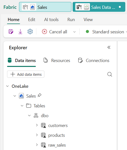
In the Explorer pane on the left, select Add to add a data source, then select your lakehouse (for example, Sales). The notebook is now attached to the lakehouse and tables you create are accessible in the Explorer pane.
-
In the notebook, run the first code cell by pressing Shift+Enter. The code creates three Delta tables in the lakehouse.
Notice that
raw_salescontains 11 rows — including a duplicate row (order_id 10 appears twice) and a null value in theregioncolumn. These quality issues are intentional and represent common problems in real source data. -
In the Explorer pane, select ↻ Refresh next to Tables to confirm that
raw_sales,customers, andproductsappear.
Shape and clean the sales data
Real-world data rarely arrives clean. In this section, you remove duplicates, handle null values, add a calculated column, and create a conditional column to categorize each order by value.
-
In the notebook, scroll to the Shape and clean the sales data section. Review the markdown cell that describes the four transformations, then run the code cell below it.
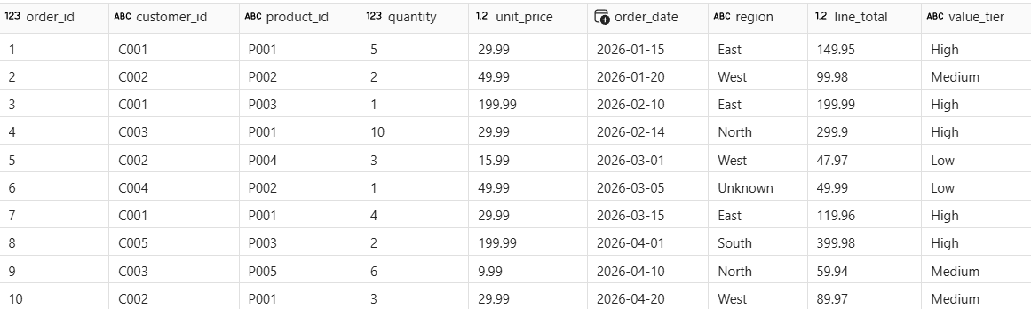
The query applies four transformations in a single pass:
SELECT DISTINCTremoves the duplicate row,COALESCEfills the null region, a calculated column computes the line total, and aCASEexpression categorizes each order by value tier. -
Run the next code cell to verify the results.
The result shows 10 rows (the duplicate is gone). The row with order_id 6 shows Unknown for region. Every row has a line_total and value_tier value.
Optionally, follow the Try it with Copilot prompt in the notebook to extend
clean_saleswith an additional column.
Join and aggregate the data
Cleansed data becomes more useful when enriched with context from other tables. In this section, you join the sales data with customer and product reference tables, then create a regional revenue summary using aggregations.
-
In the notebook, scroll to the Join and aggregate the data section and run the first code cell to join the three tables.
The
INNER JOINmatches each sales row to its customer and product details. Rows that don’t match in both tables are excluded. -
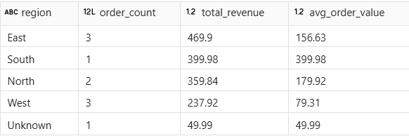
Run the next code cell to create a regional summary with aggregations.
The output shows one row per region with order counts, total revenue, and average order value. The 10 detail rows are now collapsed into summary rows — one for each region.
Optionally, follow the Try it with Copilot prompt in the notebook to create an additional aggregation by product category.
Apply window functions
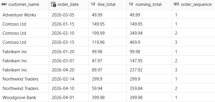
Window functions let you calculate values across related rows without collapsing the detail. In this section, you add running totals and order sequence numbers for each customer using SUM() OVER and ROW_NUMBER() OVER.
-
In the notebook, scroll to the Apply window functions section and run the code cell.
Unlike the aggregations in the previous section, the window functions keep all original rows. The
PARTITION BYclause groups rows by customer, theORDER BYclause determines the sequence, and each row gets a cumulativerunning_totaland a sequentialorder_sequencenumber.
Customers with multiple orders (like Contoso Ltd) show an increasing running total and sequential order numbers. The total row count is the same as the input.
Optionally, follow the Try it with Copilot prompt in the notebook to apply a
RANKwindow function to the data.
Write results to a Delta table
Persisting results as a Delta table makes the data available to reports, other notebooks, and downstream pipelines. In this section, you write the enriched sales view to a managed Delta table in the lakehouse.
-
In the notebook, scroll to the Write results to a Delta table section and run the first code cell.
The
CREATE OR REPLACE TABLEstatement writes the enriched view as a permanent Delta table. TheOR REPLACEoption overwrites the table if it exists, which is useful when re-running the notebook during development. -
In the Explorer pane, select ↻ Refresh next to Tables and verify that
gold_salesappears in the table list. -
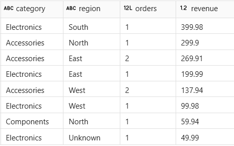
Run the next code cell to confirm the data is queryable.
The result shows revenue by product category and region, confirming that the joined and enriched data was written correctly.
Optionally, follow the Try it with Copilot prompt in the notebook to query the Delta table for high-value orders.
Clean up resources
In this exercise, you created a notebook to generate sample data, clean and shape raw sales transactions, join multiple tables, apply aggregations and window functions, and write the results to a Delta table in a Microsoft Fabric lakehouse.
If you’ve finished exploring, you can delete the workspace you created for this exercise.
-
In the bar on the left, select the icon for your workspace to view all of the items it contains.
-
In the toolbar, select Workspace settings.
-
In the General section, select Remove this workspace.