Ingest data with Spark and Microsoft Fabric notebooks
In this lab, you’ll create a Microsoft Fabric notebook and use PySpark to connect to an Azure Blob Storage path, then load the data into a lakehouse using write optimizations.
This lab will take approximately 30 minutes to complete.
For this experience, you’ll build the code across multiple notebook code cells, which may not reflect how you will do it in your environment; however, it can be useful for debugging.
Because you’re also working with a sample dataset, the optimization doesn’t reflect what you may see in production at scale; however, you can still see improvement and when every millisecond counts, optimization is key.
Note: You need a Microsoft Fabric trial to complete this exercise.
Create a workspace
Before working with data in Fabric, create a workspace with the Fabric trial enabled.
- Navigate to the Microsoft Fabric home page at
https://app.fabric.microsoft.com/home?experience=fabricin a browser and sign in with your Fabric credentials. - In the menu bar on the left, select Workspaces (the icon looks similar to 🗇).
- Create a new workspace with a name of your choice, selecting a licensing mode that includes Fabric capacity (Trial, Premium, or Fabric).
-
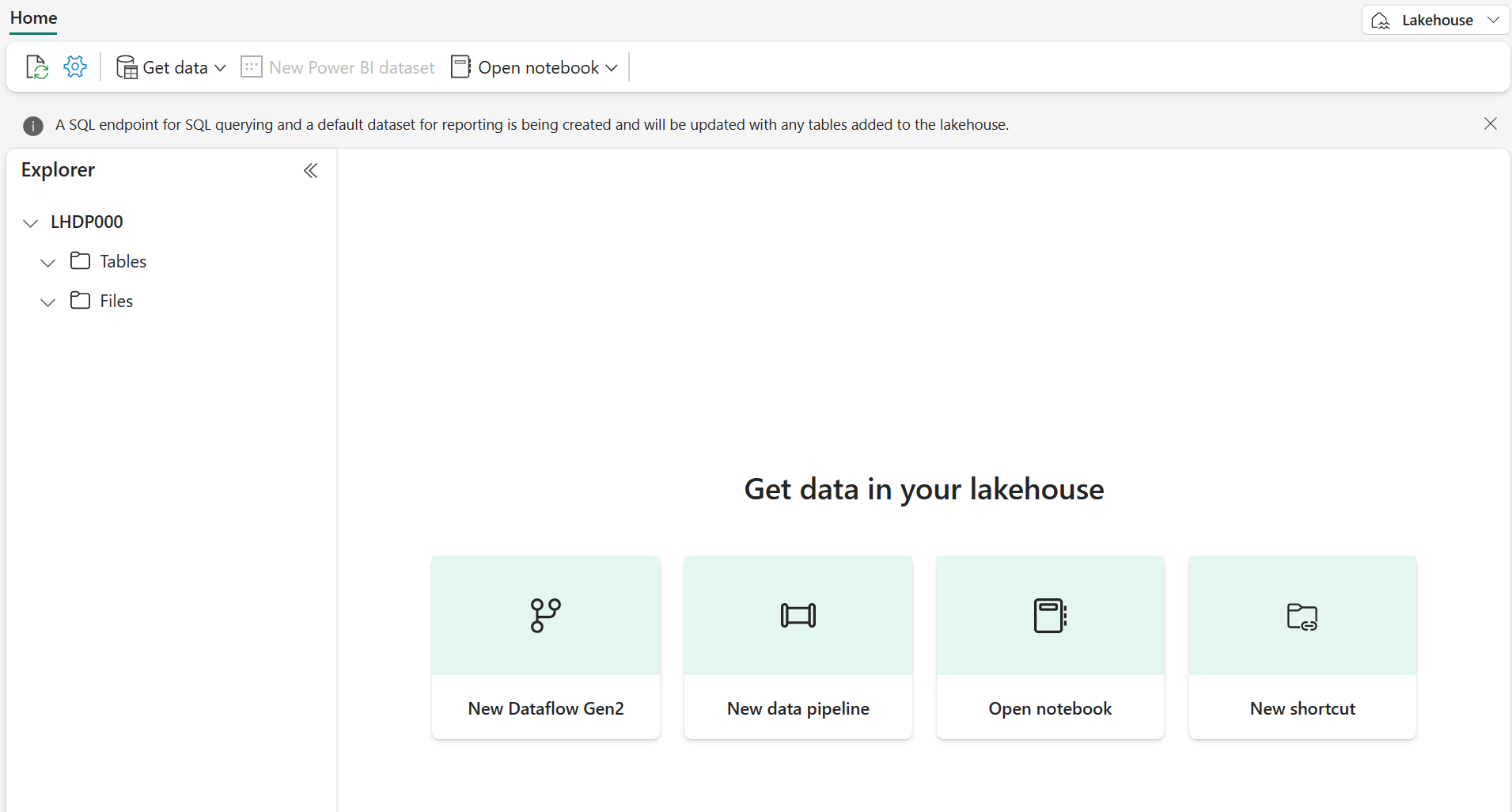
When your new workspace opens, it should be empty.
Create workspace and lakehouse destination
Start by creating a new lakehouse, and a destination folder in the lakehouse.
-
From your workspace, select + New item > Lakehouse, supply a name, and Create.
Note: It may take a few minutes to create a new lakehouse with no Tables or Files.
-
From Files, select the […] to create New subfolder named RawData.
-
From the Lakehouse Explorer within the lakehouse, select RawData > … > Properties.
-
Copy the ABFS path for the RawData folder to an empty notepad for later use, which should look something like:
abfss://{workspace_name}@onelake.dfs.fabric.microsoft.com/{lakehouse_name}.Lakehouse/Files/{folder_name}/{file_name}
You should now have a workspace with a lakehouse and a RawData destination folder.
Create a Fabric notebook and load external data
Create a new Fabric notebook and connect to external data source with PySpark.
-
From the top menu in the lakehouse, select Open notebook > New notebook, which will open once created.
Tip: You have access to the Lakehouse explorer from within this notebook, and can refresh to see progress as you complete this exercise.
-
In the default cell, notice that the code is set to PySpark (Python).
- Insert the following code into the code cell, which will:
- Declare parameters for connection string
- Build the connection string
- Read data into a DataFrame
# Azure Blob Storage access info blob_account_name = "azureopendatastorage" blob_container_name = "nyctlc" blob_relative_path = "yellow" # Construct connection path wasbs_path = f'wasbs://{blob_container_name}@{blob_account_name}.blob.core.windows.net/{blob_relative_path}' print(wasbs_path) # Read parquet data from Azure Blob Storage path blob_df = spark.read.parquet(wasbs_path) -
Select ▷ Run Cell next to the code cell to connect and read data into a DataFrame.
Expected outcome: Your command should succeed and print
wasbs://nyctlc@azureopendatastorage.blob.core.windows.net/yellowNote: A Spark session starts on the first code run, so it may take longer to complete.
-
To write the data to a file, you now need that ABFS Path for your RawData folder.
-
Insert the following code into a new code cell:
# Declare file name file_name = "yellow_taxi" # Construct destination path output_parquet_path = f"**InsertABFSPathHere**/{file_name}" print(output_parquet_path) # Load the first 1000 rows as a Parquet file blob_df.limit(1000).write.mode("overwrite").parquet(output_parquet_path) -
Add your RawData ABFS path and select ▷ Run Cell to write 1000 rows to a yellow_taxi.parquet file.
-
Your output_parquet_path should look similar to:
abfss://Spark@onelake.dfs.fabric.microsoft.com/DPDemo.Lakehouse/Files/RawData/yellow_taxi - To confirm data load from the Lakehouse Explorer, select Files > … > Refresh.
You should now see your new folder RawData with a yellow_taxi.parquet “file” - which shows as a folder with partition files within.
Transform and load data to a Delta table
Likely, your data ingestion task doesn’t end with only loading a file. Delta tables in a lakehouse allows scalable, flexible querying and storage, so we’ll create one as well.
-
Create a new code cell, and insert the following code:
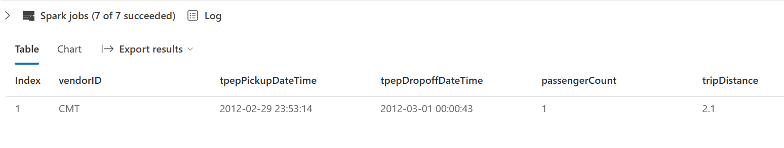
from pyspark.sql.functions import col, to_timestamp, current_timestamp, year, month # Read the parquet data from the specified path raw_df = spark.read.parquet(output_parquet_path) # Add dataload_datetime column with current timestamp filtered_df = raw_df.withColumn("dataload_datetime", current_timestamp()) # Filter columns to exclude any NULL values in storeAndFwdFlag filtered_df = filtered_df.filter(col("storeAndFwdFlag").isNotNull()) # Load the filtered data into a Delta table table_name = "yellow_taxi" filtered_df.write.format("delta").mode("append").saveAsTable(table_name) # Display results display(filtered_df.limit(1)) -
Select ▷ Run Cell next to the code cell.
- This will add a timestamp column dataload_datetime to log when the data was loaded to a Delta table
- Filter NULL values in storeAndFwdFlag
- Load filtered data into a Delta table
- Display a single row for validation
-
Review and confirm the displayed results, something similar to the following image:
You’ve now successfully connected to external data, written it to a parquet file, loaded the data into a DataFrame, transformed the data, and loaded it to a Delta table.
Analyze Delta table data with SQL queries
This lab is focused on data ingestion, which really explains the extract, transform, load process, but it’s valuable for you to preview the data too.
-
Create a new code cell, and insert the code below:
# Load table into df delta_table_name = "yellow_taxi" table_df = spark.read.format("delta").table(delta_table_name) # Create temp SQL table table_df.createOrReplaceTempView("yellow_taxi_temp") # SQL Query table_df = spark.sql('SELECT * FROM yellow_taxi_temp') # Display 10 results display(table_df.limit(10)) -
Select ▷ Run Cell next to the code cell.
Many data analysts are comfortable working with SQL syntax. Spark SQL is a SQL language API in Spark that you can use to run SQL statements, or even persist data in relational tables.
The code you just ran creates a relational view of the data in a dataframe, and then uses the spark.sql library to embed Spark SQL syntax within your Python code and query the view and return the results as a dataframe.
Clean up resources
In this exercise, you have used notebooks with PySpark in Fabric to load data and save it to Parquet. You then used that Parquet file to further transform the data. Finally you used SQL to query the Delta tables.
When you’re finished exploring, you can delete the workspace you created for this exercise.
- In the bar on the left, select the icon for your workspace to view all of the items it contains.
- Select Workspace settings and in the General section, scroll down and select Remove this workspace.
- Select Delete to delete the workspace.