Train and track machine learning models with MLflow in Microsoft Fabric
In this lab, you’ll train a machine learning model to predict a quantitative measure of diabetes. You’ll train a regression model with scikit-learn, and track and compare your models with MLflow.
By completing this lab, you’ll gain hands-on experience in machine learning and model tracking, and learn how to work with notebooks, experiments, and models in Microsoft Fabric.
This lab will take approximately 25 minutes to complete.
Create a workspace
Note: You need access to a Fabric paid or trial capacity to complete this exercise. For information about the free Fabric trial, see Fabric trial.
- Navigate to theMicrosoft Fabric home page at
https://app.fabric.microsoft.com/home?experience=fabricin a browser and sign in with your Fabric credentials. - In the menu bar on the left, select Workspaces (the icon looks similar to 🗇).
- Create a new workspace with a name of your choice, selecting a licensing mode that includes Fabric capacity (Trial, Premium, or Fabric).
-
When your new workspace opens, it should be empty.
Create a notebook
To train a model, you can create a notebook. Notebooks provide an interactive environment in which you can write and run code (in multiple languages).
-
In the menu bar on the left, select Create. In the New page, under the Data Science section, select Notebook. Give it a unique name of your choice.
Note: If the Create option is not pinned to the sidebar, you need to select the ellipsis (…) option first.
After a few seconds, a new notebook containing a single cell will open. Notebooks are made up of one or more cells that can contain code or markdown (formatted text).
-
Select the first cell (which is currently a code cell), and then in the dynamic tool bar at its top-right, use the M↓ button to convert the cell to a markdown cell.
When the cell changes to a markdown cell, the text it contains is rendered.
-
If necessary, use the 🖉 (Edit) button to switch the cell to editing mode, then delete the content and enter the following text:
# Train a machine learning model and track with MLflow
Load data into a dataframe
Now you’re ready to run code to get data and train a model. You’ll work with the diabetes dataset from the Azure Open Datasets. After loading the data, you’ll convert the data to a Pandas dataframe: a common structure for working with data in rows and columns.
-
In your notebook, use the + Code icon below the latest cell output to add a new code cell to the notebook.
Tip: To see the + Code icon, move the mouse to just below and to the left of the output from the current cell. Alternatively, in the menu bar, on the Edit tab, select + Add code cell.
-
Enter the following code in it:
# Azure storage access info for open dataset diabetes blob_account_name = "azureopendatastorage" blob_container_name = "mlsamples" blob_relative_path = "diabetes" blob_sas_token = r"" # Blank since container is Anonymous access # Set Spark config to access blob storage wasbs_path = f"wasbs://%s@%s.blob.core.windows.net/%s" % (blob_container_name, blob_account_name, blob_relative_path) spark.conf.set("fs.azure.sas.%s.%s.blob.core.windows.net" % (blob_container_name, blob_account_name), blob_sas_token) print("Remote blob path: " + wasbs_path) # Spark read parquet, note that it won't load any data yet by now df = spark.read.parquet(wasbs_path) -
Use the ▷ Run cell button on the left of the cell to run it. Alternatively, you can press SHIFT + ENTER on your keyboard to run a cell.
Note: Since this is the first time you’ve run any Spark code in this session, the Spark pool must be started. This means that the first run in the session can take a minute or so to complete. Subsequent runs will be quicker.
-
Use the + Code icon below the cell output to add a new code cell to the notebook, and enter the following code in it:
display(df) -
When the cell command has completed, review the output below the cell, which should look similar to this:
AGE SEX BMI BP S1 S2 S3 S4 S5 S6 Y 59 2 32.1 101.0 157 93.2 38.0 4.0 4.8598 87 151 48 1 21.6 87.0 183 103.2 70.0 3.0 3.8918 69 75 72 2 30.5 93.0 156 93.6 41.0 4.0 4.6728 85 141 24 1 25.3 84.0 198 131.4 40.0 5.0 4.8903 89 206 50 1 23.0 101.0 192 125.4 52.0 4.0 4.2905 80 135 … … … … … … … … … … … The output shows the rows and columns of the diabetes dataset.
-
The data is loaded as a Spark dataframe. Scikit-learn will expect the input dataset to be a Pandas dataframe. Run the code below to convert your dataset to a Pandas dataframe:
import pandas as pd
df = df.toPandas()
df.head()
Train a machine learning model
Now that you’ve loaded the data, you can use it to train a machine learning model and predict a quantitative measure of diabetes. You’ll train a regression model using the scikit-learn library and track the model with MLflow.
-
Run the following code to split the data into a training and test dataset, and to separate the features from the label you want to predict:
from sklearn.model_selection import train_test_split X, y = df[['AGE','SEX','BMI','BP','S1','S2','S3','S4','S5','S6']].values, df['Y'].values X_train, X_test, y_train, y_test = train_test_split(X, y, test_size=0.30, random_state=0) -
Add another new code cell to the notebook, enter the following code in it, and run it:
import mlflow
experiment_name = "experiment-diabetes"
mlflow.set_experiment(experiment_name)
The code creates an MLflow experiment named experiment-diabetes. Your models will be tracked in this experiment.
-
Add another new code cell to the notebook, enter the following code in it, and run it:
from sklearn.linear_model import LinearRegression

with mlflow.start_run():
   mlflow.autolog()

   model = LinearRegression()
   model.fit(X_train, y_train)

   mlflow.log_param("estimator", "LinearRegression")
The code trains a regression model using Linear Regression. Parameters, metrics, and artifacts, are automatically logged with MLflow. Additionally, you’re logging a parameter called estimator with the value LinearRegression.
-
Add another new code cell to the notebook, enter the following code in it, and run it:
from sklearn.tree import DecisionTreeRegressor

with mlflow.start_run():
   mlflow.autolog()

   model = DecisionTreeRegressor(max_depth=5)
   model.fit(X_train, y_train)

   mlflow.log_param("estimator", "DecisionTreeRegressor")
The code trains a regression model using Decision Tree Regressor. Parameters, metrics, and artifacts, are automatically logged with MLflow. Additionally, you’re logging a parameter called estimator with the value DecisionTreeRegressor.
Use MLflow to search and view your experiments
When you’ve trained and tracked models with MLflow, you can use the MLflow library to retrieve your experiments and its details.
-
To list all experiments, use the following code:
import mlflow experiments = mlflow.search_experiments() for exp in experiments: print(exp.name) -
To retrieve a specific experiment, you can get it by its name:
experiment_name = "experiment-diabetes" exp = mlflow.get_experiment_by_name(experiment_name) print(exp) -
Using an experiment name, you can retrieve all jobs of that experiment:
mlflow.search_runs(exp.experiment_id) -
To more easily compare job runs and outputs, you can configure the search to order the results. For example, the following cell orders the results by start_time, and only shows a maximum of 2 results:
mlflow.search_runs(exp.experiment_id, order_by=["start_time DESC"], max_results=2) -
Finally, you can plot the evaluation metrics of multiple models next to each other to easily compare models:
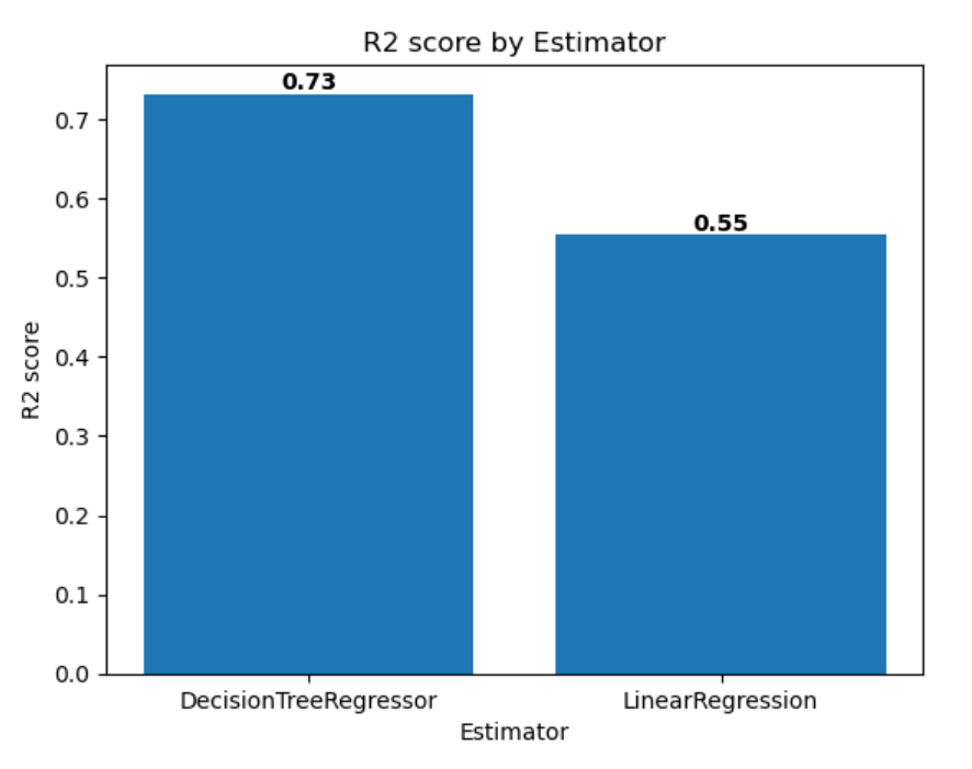
import matplotlib.pyplot as plt

df_results = mlflow.search_runs(exp.experiment_id, order_by=["start_time DESC"], max_results=2)[["metrics.training_r2_score", "params.estimator"]]

fig, ax = plt.subplots()
ax.bar(df_results["params.estimator"], df_results["metrics.training_r2_score"])
ax.set_xlabel("Estimator")
ax.set_ylabel("R2 score")
ax.set_title("R2 score by Estimator")
for i, v in enumerate(df_results["metrics.training_r2_score"]):
    ax.text(i, v, str(round(v, 2)), ha='center', va='bottom', fontweight='bold')
plt.show()
The output should resemble the following image:
Explore your experiments
Microsoft Fabric will keep track of all your experiments and allows you to visually explore them.
- Navigate to your workspace from the menu bar on the left.
-
Select the experiment-diabetes experiment to open it.
Tip: If you don’t see any logged experiment runs, refresh the page.
- Select the View tab.
- Select Run list.
-
Select the two latest runs by checking each box.
As a result, your two last runs will be compared to each other in the Metric comparison pane. By default, the metrics are plotted by run name.
- Select the 🖉 (Edit) button of the graph visualizing the mean absolute error for each run.
- Change the visualization type to bar.
- Change the X-axis to estimator.
- Select Replace and explore the new graph.
- Optionally, you can repeat these steps for the other graphs in the Metric comparison pane.
By plotting the performance metrics per logged estimator, you can review which algorithm resulted in a better model.
Save the model
After comparing machine learning models that you’ve trained across experiment runs, you can choose the best performing model. To use the best performing model, save the model and use it to generate predictions.
- In the experiment overview, ensure the View tab is selected.
- Select Run details.
- Select the run with the highest Training R2 score.
- Select Save in the Save run as model box (you may need to scroll to the right to see this).
- Select Create a new model in the newly opened pop-up window.
- Select the model folder.
- Name the model
model-diabetes, and select Save. - Select View ML model in the notification that appears at the top right of your screen when the model is created. You can also refresh the window. The saved model is linked under Model versions.
Note that the model, the experiment, and the experiment run are linked, allowing you to review how the model is trained.
Save the notebook and end the Spark session
Now that you’ve finished training and evaluating the models, you can save the notebook with a meaningful name and end the Spark session.
- Return to your notebook, and, in the notebook menu bar, use the ⚙️ Settings icon to view the notebook settings.
- Set the Name of the notebook to Train and compare models, and then close the settings pane.
- On the notebook menu, select Stop session to end the Spark session.
Clean up resources
In this exercise, you have created a notebook and trained a machine learning model. You used scikit-learn to train the model and MLflow to track its performance.
If you’ve finished exploring your model and experiments, you can delete the workspace that you created for this exercise.
- In the bar on the left, select the icon for your workspace to view all of the items it contains.
- In the … menu on the toolbar, select Workspace settings.
- In the General section, select Remove this workspace .