Get started with data science in Microsoft Fabric

In this lab, you’ll ingest data, explore the data in a notebook, process the data with the Data Wrangler, and train two types of models. By performing all these steps, you’ll be able to explore the data science features in Microsoft Fabric.

By completing this lab, you’ll gain hands-on experience in machine learning and model tracking, and learn how to work with notebooks, Data Wrangler, experiments, and models in Microsoft Fabric.

This lab will take approximately 20 minutes to complete.

Note: You need a Microsoft Fabric trial to complete this exercise.

Create a workspace

Before working with data in Fabric, create a workspace with the Fabric trial enabled.

Navigate to the Microsoft Fabric home page at https://app.fabric.microsoft.com in a browser.
Select Synapse Data Science.
In the menu bar on the left, select Workspaces (the icon looks similar to 🗇).
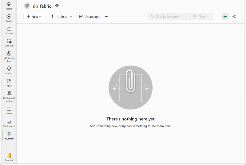
Create a new workspace with a name of your choice, selecting a licensing mode that includes Fabric capacity (Trial, Premium, or Fabric).
When your new workspace opens, it should be empty.

Create a notebook

To run code, you can create a notebook. Notebooks provide an interactive environment in which you can write and run code (in multiple languages).

In the Synapse Data Science home page, create a new Notebook.

After a few seconds, a new notebook containing a single cell will open. Notebooks are made up of one or more cells that can contain code or markdown (formatted text).
Select the first cell (which is currently a code cell), and then in the dynamic tool bar at its top-right, use the M↓ button to convert the cell to a markdown cell.

When the cell changes to a markdown cell, the text it contains is rendered.
Use the 🖉 (Edit) button to switch the cell to editing mode, then delete the content and enter the following text:
```
# Data science in Microsoft Fabric
```

Get the data

Now you’re ready to run code to get data and train a model. You’ll work with the diabetes dataset from the Azure Open Datasets. After loading the data, you’ll convert the data to a Pandas dataframe: a common structure for working with data in rows and columns.

In your notebook, use the + Code icon below the latest cell output to add a new code cell to the notebook.

Tip: To see the + Code icon, move the mouse to just below and to the left of the output from the current cell. Alternatively, in the menu bar, on the Edit tab, select + Add code cell.

Enter the following code in the new code cell:

# Azure storage access info for open dataset diabetes
blob_account_name = "azureopendatastorage"
blob_container_name = "mlsamples"
blob_relative_path = "diabetes"
blob_sas_token = r"" # Blank since container is Anonymous access
    
# Set Spark config to access  blob storage
wasbs_path = f"wasbs://%s@%s.blob.core.windows.net/%s" % (blob_container_name, blob_account_name, blob_relative_path)
spark.conf.set("fs.azure.sas.%s.%s.blob.core.windows.net" % (blob_container_name, blob_account_name), blob_sas_token)
print("Remote blob path: " + wasbs_path)
    
# Spark read parquet, note that it won't load any data yet by now
df = spark.read.parquet(wasbs_path)

Use the ▷ Run cell button on the left of the cell to run it. Alternatively, you can press SHIFT + ENTER on your keyboard to run a cell.

Note: Since this is the first time you’ve run any Spark code in this session, the Spark pool must be started. This means that the first run in the session can take a minute or so to complete. Subsequent runs will be quicker.
Use the + Code icon below the cell output to add a new code cell to the notebook, and enter the following code in it:
```
display(df)
```

When the cell command has completed, review the output below the cell, which should look similar to this:

AGE	SEX	BMI	BP	S1	S2	S3	S4	S5	S6	Y
59	2	32.1	101.0	157	93.2	38.0	4.0	4.8598	87	151
48	1	21.6	87.0	183	103.2	70.0	3.0	3.8918	69	75
72	2	30.5	93.0	156	93.6	41.0	4.0	4.6728	85	141
24	1	25.3	84.0	198	131.4	40.0	5.0	4.8903	89	206
50	1	23.0	101.0	192	125.4	52.0	4.0	4.2905	80	135
…	…	…	…	…	…	…	…	…	…	…

The output shows the rows and columns of the diabetes dataset.

There are two tabs at the top of the rendered table: Table and Chart. Select Chart.
Select the View options at the right top of the chart to change the visualization.
Change the chart to the following settings:
- Chart Type: Box plot
- Key: Leave empty
- Values: Y
Select Apply to render the new visualization and explore the output.

Prepare the data

Now that you have ingested and explored the data, you can transform the data. You can either run code in a notebook, or use the Data Wrangler to generate code for you.

The data is loaded as a Spark dataframe. To launch the Data Wrangler, you need to convert the data to a Pandas dataframe. Run the following code in your notebook:
```
df = df.toPandas()
df.head()
```
Select Data in the notebook ribbon, and then select Transform DataFrame in Data Wrangler dropdown.
Select the df dataset. When Data Wrangler launches, it generates a descriptive overview of the dataframe in the Summary panel.

Currently, the label column is Y, which is a continuous variable. To train a machine learning model that predicts Y, you need to train a regression model. The (predicted) values of Y may be difficult to interpret. Instead, we could explore training a classification model which predicts whether someone is low risk or high risk for developing diabetes. To be able to train a classification model, you need to create a binary label column based on the values from Y.
Select the Y column in the Data Wrangler. Note that there is a decrease in frequency for the 220-240 bin. The 75th percentile 211.5 roughly aligns with transition of the two regions in the histogram. Let’s use this value as the threshold for low and high risk.
Navigate to the Operations panel, expand Formulas, and then select Create column from formula.
Create a new column with the following settings:
- Column name: Risk
- Column formula: (df['Y'] > 211.5).astype(int)
Review the new column Risk that is added to the preview. Verify that the count of rows with value 1 should be roughly 25% of all rows (as it’s the 75th percentile of Y).
Select Apply.
Select Add code to notebook.
Run the cell with the code that is generated by Data Wrangler.
Run the following code in a new cell to verify that the Risk column is shaped as expected:
```
df_clean.describe()
```

Train machine learning models

Now that you’ve prepared the data, you can use it to train a machine learning model to predict diabetes. We can train two different types of models with our dataset: a regression model (predicting Y) or a classification model (predicting Risk). You’ll train the models using the scikit-learn library and track the models with MLflow.

Train a regression model

Run the following code to split the data into a training and test dataset, and to separate the features from the label Y you want to predict:

from sklearn.model_selection import train_test_split
    
X, y = df_clean[['AGE','SEX','BMI','BP','S1','S2','S3','S4','S5','S6']].values, df_clean['Y'].values
    
X_train, X_test, y_train, y_test = train_test_split(X, y, test_size=0.30, random_state=0)

Add another new code cell to the notebook, enter the following code in it, and run it:
```
import mlflow
experiment_name = "diabetes-regression"
mlflow.set_experiment(experiment_name)
```
The code creates an MLflow experiment named diabetes-regression. Your models will be tracked in this experiment.
Add another new code cell to the notebook, enter the following code in it, and run it:
```
from sklearn.linear_model import LinearRegression
    
with mlflow.start_run():
   mlflow.autolog()
    
   model = LinearRegression()
   model.fit(X_train, y_train)
```
The code trains a regression model using Linear Regression. Parameters, metrics, and artifacts, are automatically logged with MLflow.

Train a classification model

Run the following code to split the data into a training and test dataset, and to separate the features from the label Risk you want to predict:

from sklearn.model_selection import train_test_split
    
X, y = df_clean[['AGE','SEX','BMI','BP','S1','S2','S3','S4','S5','S6']].values, df_clean['Risk'].values
    
X_train, X_test, y_train, y_test = train_test_split(X, y, test_size=0.30, random_state=0)

Add another new code cell to the notebook, enter the following code in it, and run it:
```
import mlflow
experiment_name = "diabetes-classification"
mlflow.set_experiment(experiment_name)
```
The code creates an MLflow experiment named diabetes-classification. Your models will be tracked in this experiment.
Add another new code cell to the notebook, enter the following code in it, and run it:
```
from sklearn.linear_model import LogisticRegression
    
with mlflow.start_run():
    mlflow.sklearn.autolog()

    model = LogisticRegression(C=1/0.1, solver="liblinear").fit(X_train, y_train)
```
The code trains a classification model using Logistic Regression. Parameters, metrics, and artifacts, are automatically logged with MLflow.

Explore your experiments

Microsoft Fabric will keep track of all your experiments and allows you to visually explore them.

Navigate to your workspace from the hub menu bar on the left.
Select the diabetes-regression experiment to open it.

Tip: If you don’t see any logged experiment runs, refresh the page.
Review the Run metrics to explore accurate your regression model is.
Navigate back to the home page and select the diabetes-classification experiment to open it.
Review the Run metrics to explore the accuracy of the classification model. Note that the type of metrics are different as you trained a different type of model.

Save the model

After comparing machine learning models that you’ve trained across experiments, you can choose the best performing model. To use the best performing model, save the model and use it to generate predictions.

Select Save as ML model in the experiment ribbon.
Select Create a new ML model in the newly opened pop-up window.
Select the model folder.
Name the model model-diabetes, and select Save.
Select View ML model in the notification that appears at the top right of your screen when the model is created. You can also refresh the window. The saved model is linked under ML model versions.

Note that the model, the experiment, and the experiment run are linked, allowing you to review how the model is trained.

Save the notebook and end the Spark session

Now that you’ve finished training and evaluating the models, you can save the notebook with a meaningful name and end the Spark session.

In the notebook menu bar, use the ⚙️ Settings icon to view the notebook settings.
Set the Name of the notebook to Train and compare models, and then close the settings pane.
On the notebook menu, select Stop session to end the Spark session.

Clean up resources

In this exercise, you have created a notebook and trained a machine learning model. You used scikit-learn to train the model and MLflow to track its performance.

If you’ve finished exploring your model and experiments, you can delete the workspace that you created for this exercise.

In the bar on the left, select the icon for your workspace to view all of the items it contains.
In the … menu on the toolbar, select Workspace settings.
In the General section, select Remove this workspace .