Create a Microsoft Fabric Lakehouse
Large-scale data analytics solutions have traditionally been built around a data warehouse, in which data is stored in relational tables and queried using SQL. The growth in “big data” (characterized by high volumes, variety, and velocity of new data assets) together with the availability of low-cost storage and cloud-scale distributed compute technologies has led to an alternative approach to analytical data storage; the data lake. In a data lake, data is stored as files without imposing a fixed schema for storage. Increasingly, data engineers and analysts seek to benefit from the best features of both of these approaches by combining them in a data lakehouse; in which data is stored in files in a data lake and a relational schema is applied to them as a metadata layer so that they can be queried using traditional SQL semantics.
In Microsoft Fabric, a lakehouse provides highly scalable file storage in a OneLake store (built on Azure Data Lake Store Gen2) with a metastore for relational objects such as tables and views based on the open source Delta Lake table format. Delta Lake enables you to define a schema of tables in your lakehouse that you can query using SQL.
This lab takes approximately 30 minutes to complete.
Tip: For related training content, see Get started with lakehouses in Microsoft Fabric.
Create a workspace
Note: You need access to a Fabric paid or trial capacity to complete this exercise. For information about the free Fabric trial, see Fabric trial.
- Navigate to the Microsoft Fabric home page at
https://app.fabric.microsoft.com/home?experience=fabricin a browser, and sign in with your Fabric credentials. - In the menu bar on the left, select Workspaces (the icon looks similar to 🗇).
- Create a new workspace with a name of your choice, selecting a licensing mode in the Advanced section that includes Fabric capacity (Trial, Premium, or Fabric).
-
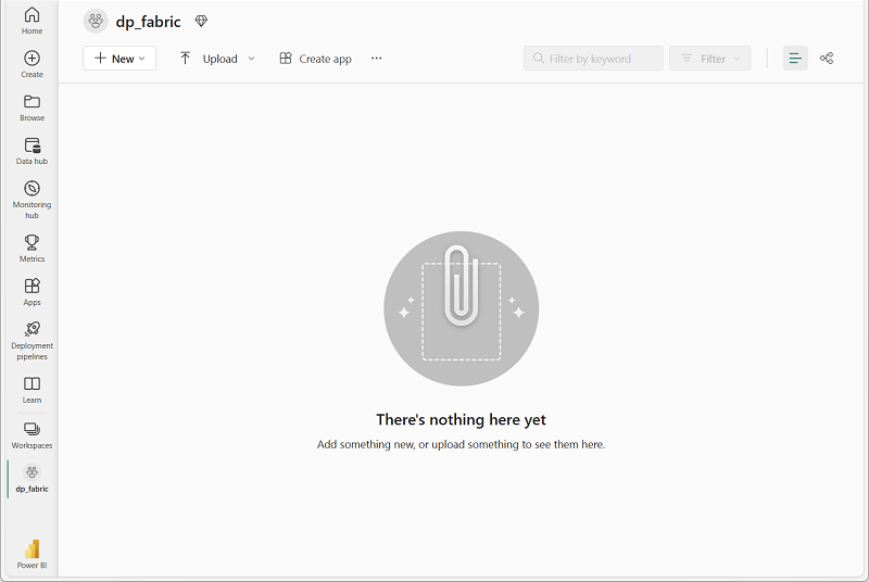
When your new workspace opens, it should be empty.
Create a lakehouse
Now that you have a workspace, it’s time to create a data lakehouse for your data files.
-
On the menu bar on the left, select Create. In the New page, under the Data Engineering section, select Lakehouse. Give it a unique name of your choice.
Note: If the Create option is not pinned to the sidebar, you need to select the ellipsis (…) option first.
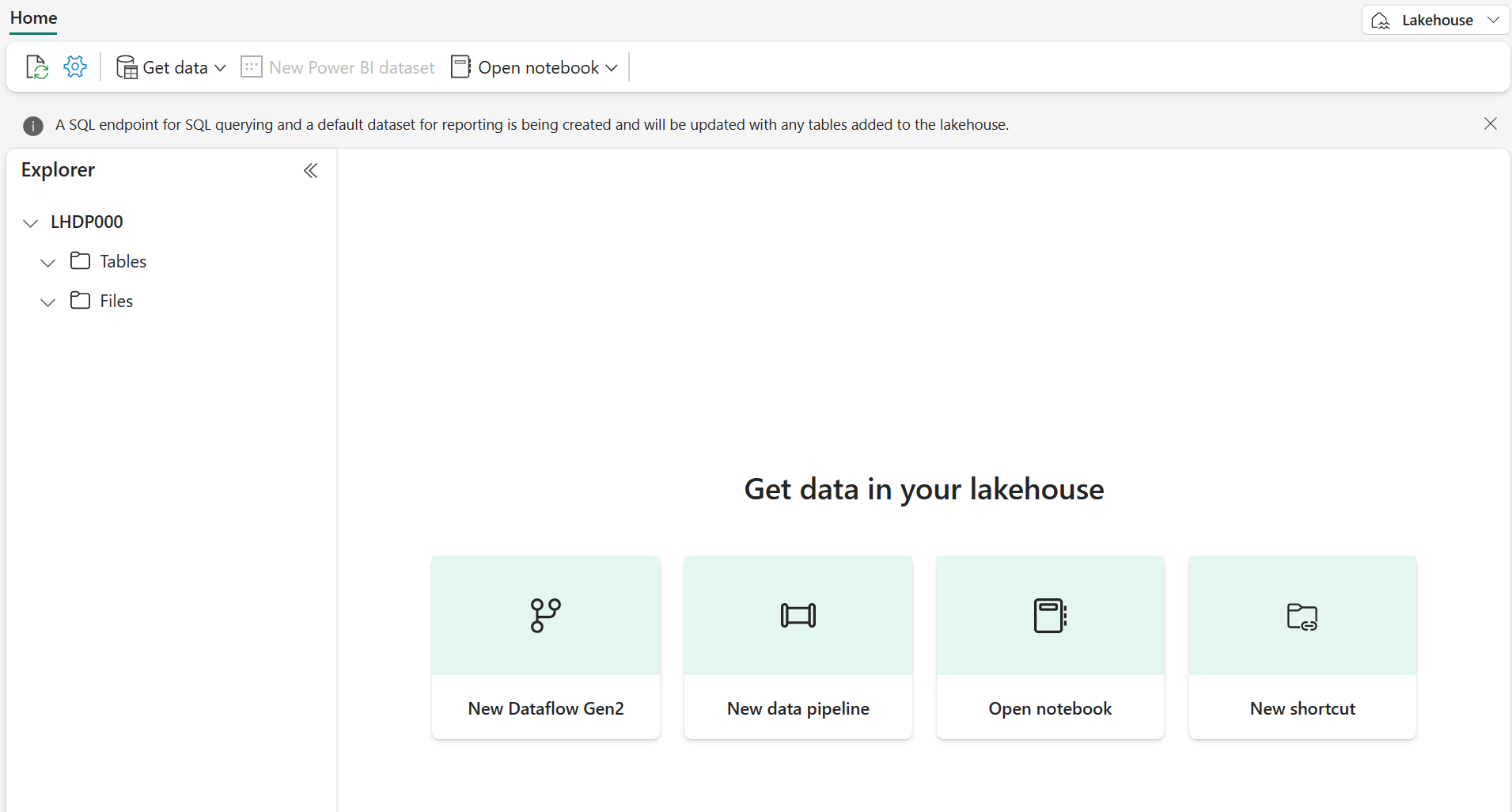
After a minute or so, a new lakehouse will be created:
-
View the new lakehouse, and note that the Lakehouse explorer pane on the left enables you to browse tables and files in the lakehouse:
- The Tables folder contains tables that you can query using SQL semantics. Tables in a Microsoft Fabric lakehouse are based on the open source Delta Lake file format, commonly used in Apache Spark.
- The Files folder contains data files in the OneLake storage for the lakehouse that aren’t associated with managed delta tables. You can also create shortcuts in this folder to reference data that is stored externally.
Currently, there are no tables or files in the lakehouse.
Upload a file
Fabric provides multiple ways to load data into the lakehouse, including built-in support for pipelines that copy data from external sources and data flows (Gen 2) that you can define using visual tools based on Power Query. However one of the simplest ways to ingest small amounts of data is to upload files or folders from your local computer (or lab VM if applicable).
-
Download the sales.csv file from
https://raw.githubusercontent.com/MicrosoftLearning/dp-data/main/sales.csv, saving it as sales.csv on your local computer (or lab VM if applicable).Note: To download the file, open a new tab in the browser and paste in the URL. Right click anywhere on the page containing the data and select Save as to save the page as a CSV file.
- Return to the web browser tab containing your lakehouse, and in the … menu for the Files folder in the Explorer pane, select New subfolder, and create a subfolder named data.
- In the … menu for the new data folder, select Upload and Upload files, and then upload the sales.csv file from your local computer (or lab VM if applicable).
-
After the file has been uploaded, select the Files/data folder and verify that the sales.csv file has been uploaded, as shown here:
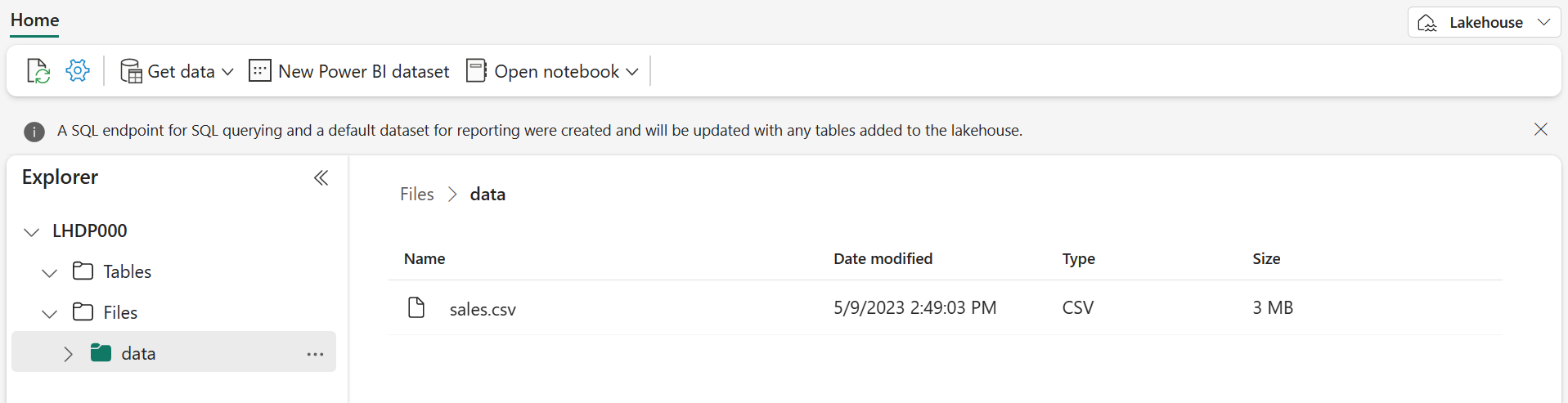
- Select the sales.csv file to see a preview of its contents.
Explore shortcuts
In many scenarios, the data you need to work with in your lakehouse may be stored in some other location. While there are many ways to ingest data into the OneLake storage for your lakehouse, another option is to instead create a shortcut. Shortcuts enable you to include externally sourced data in your analytics solution without the overhead and risk of data inconsistency associated with copying it.
- In the … menu for the Files folder, select New shortcut.
- View the available data source types for shortcuts. Then close the New shortcut dialog box without creating a shortcut.
Load file data into a table
The sales data you uploaded is in a file, which data analysts and engineers can work with directly by using Apache Spark code. However, in many scenarios you may want to load the data from the file into a table so that you can query it using SQL.
- In the Explorer pane, select the Files/data folder so you can see the sales.csv file it contains.
- In the … menu for the sales.csv file, select Load to Tables > New table.
- In Load to table dialog box, set the table name to
salesand confirm the load operation. Then wait for the table to be created and loaded. -
Select CSV for the file type. Then wait for the table to be created and loaded.
Tip: If the
salestable does not automatically appear, in the … menu for the Tables folder, select Refresh. -
In the Explorer pane, select the
salestable that has been created to view the data.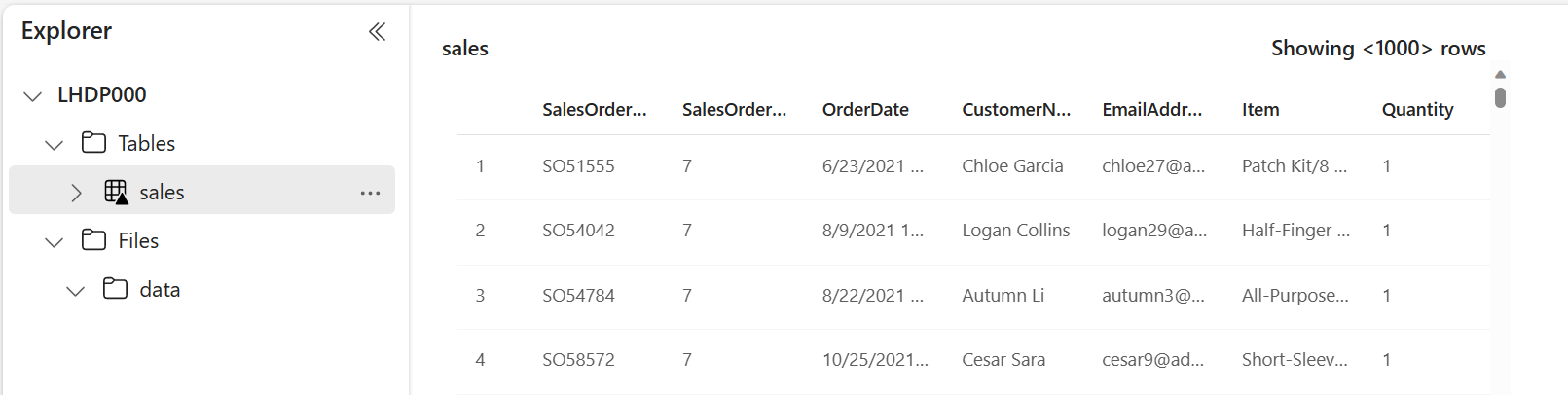
-
In the … menu for the
salestable, select View files to see the underlying files for this table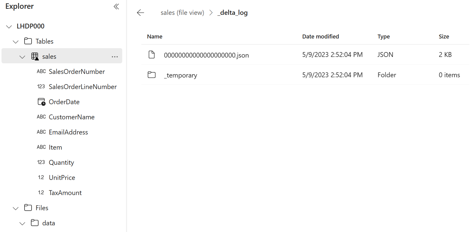
Files for a delta table are stored in Parquet format, and include a subfolder named _delta_log in which details of transactions applied to the table are logged.
Use SQL to query tables
When you create a lakehouse and define tables in it, a SQL endpoint is automatically created through which the tables can be queried using SQL SELECT statements.
-
At the top-right of the Lakehouse page, switch from Lakehouse to SQL analytics endpoint. Then wait a short time until the SQL analytics endpoint for your lakehouse opens in a visual interface from which you can query its tables.
-
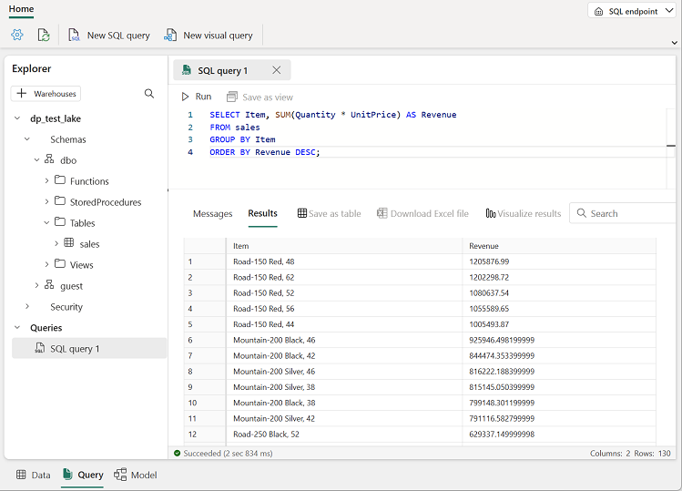
Use the New SQL query button to open a new query editor, and enter the following SQL query:
SELECT Item, SUM(Quantity * UnitPrice) AS Revenue FROM sales GROUP BY Item ORDER BY Revenue DESC;Note: If you are in a lab VM and have any problems entering the SQL query, you can download the 01-Snippets.txt file from
https://github.com/MicrosoftLearning/mslearn-fabric/raw/main/Allfiles/Labs/01/Assets/01-Snippets.txt, saving it on the VM. You can then copy the query from the text file. -
Use the ▷ Run button to run the query and view the results, which should show the total revenue for each product.
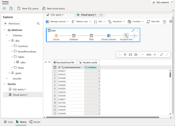
Create a visual query
While many data professionals are familiar with SQL, data analysts with Power BI experience can apply their Power Query skills to create visual queries.
- On the toolbar, expand the New SQL query option and select New visual query.
-
Drag the
salestable to the new visual query editor pane that opens to create a Power Query as shown here: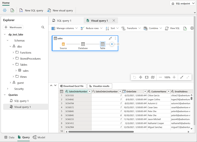
-
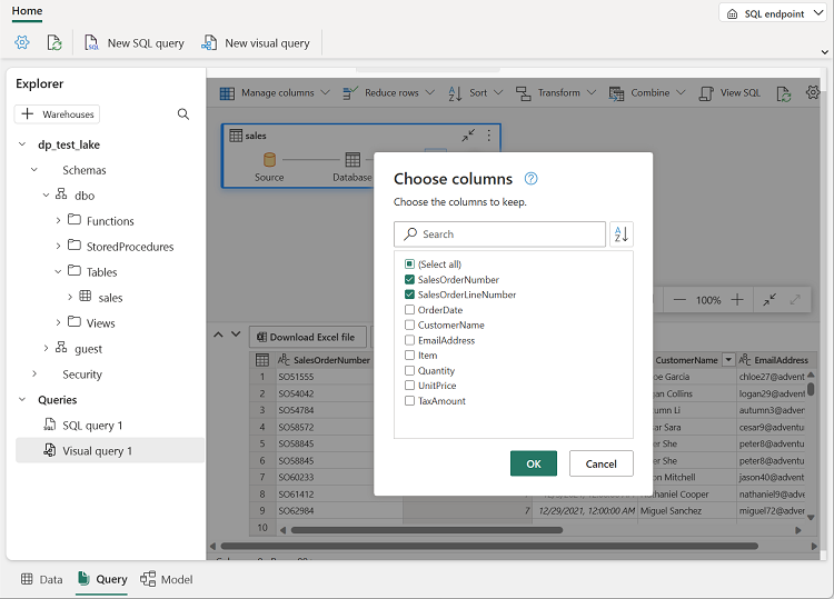
In the Manage columns menu, select Choose columns. Then select only the SalesOrderNumber and SalesOrderLineNumber columns.
-
in the Transform menu, select Group by. Then group the data by using the following Basic settings:
- Group by: SalesOrderNumber
- New column name: LineItems
- Operation: Count distinct values
- Column: SalesOrderLineNumber
When you’re done, the results pane under the visual query shows the number of line items for each sales order.
Clean up resources
In this exercise, you have created a lakehouse and imported data into it. You’ve seen how a lakehouse consists of files and tables stored in a OneLake data store. The managed tables can be queried using SQL.
If you’ve finished exploring your lakehouse, you can delete the workspace you created for this exercise.
- In the bar on the left, select the icon for your workspace to view all of the items it contains.
- In the toolbar, select Workspace settings.
- In the General section, select Remove this workspace.