Train a deep learning model

In this exercise, you’ll use the PyTorch library to train a deep learning model in Azure Databricks. Then you’ll use the Horovod library to distribute deep learning training across multiple worker nodes in a cluster.

This exercise should take approximately 45 minutes to complete.

Before you start

You’ll need an Azure subscription in which you have administrative-level access.

Provision an Azure Databricks workspace

Tip: If you already have an Azure Databricks workspace, you can skip this procedure and use your existing workspace.

This exercise includes a script to provision a new Azure Databricks workspace. The script attempts to create a Premium tier Azure Databricks workspace resource in a region in which your Azure subscription has sufficient quota for the compute cores required in this exercise; and assumes your user account has sufficient permissions in the subscription to create an Azure Databricks workspace resource. If the script fails due to insufficient quota or permissions, you can try to create an Azure Databricks workspace interactively in the Azure portal.

In a web browser, sign into the Azure portal at https://portal.azure.com.
Use the [>_] button to the right of the search bar at the top of the page to create a new Cloud Shell in the Azure portal, selecting a PowerShell environment and creating storage if prompted. The cloud shell provides a command line interface in a pane at the bottom of the Azure portal, as shown here:

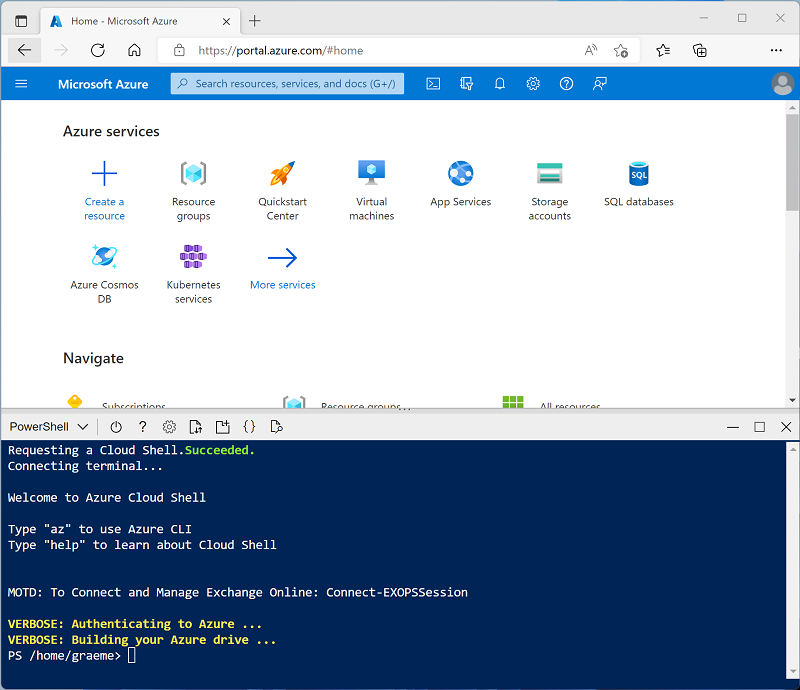
Note: If you have previously created a cloud shell that uses a Bash environment, use the the drop-down menu at the top left of the cloud shell pane to change it to PowerShell.
Note that you can resize the cloud shell by dragging the separator bar at the top of the pane, or by using the —, ◻, and X icons at the top right of the pane to minimize, maximize, and close the pane. For more information about using the Azure Cloud Shell, see the Azure Cloud Shell documentation.

In the PowerShell pane, enter the following commands to clone this repo:

 rm -r mslearn-databricks -f
 git clone https://github.com/MicrosoftLearning/mslearn-databricks

After the repo has been cloned, enter the following command to run the setup.ps1 script, which provisions an Azure Databricks workspace in an available region:
```
 ./mslearn-databricks/setup.ps1
```
If prompted, choose which subscription you want to use (this will only happen if you have access to multiple Azure subscriptions).
Wait for the script to complete - this typically takes around 5 minutes, but in some cases may take longer. While you are waiting, review the Distributed training article in the Azure Databricks documentation.

Create a cluster

Azure Databricks is a distributed processing platform that uses Apache Spark clusters to process data in parallel on multiple nodes. Each cluster consists of a driver node to coordinate the work, and worker nodes to perform processing tasks. In this exercise, you’ll create a single-node cluster to minimize the compute resources used in the lab environment (in which resources may be constrained). In a production environment, you’d typically create a cluster with multiple worker nodes.

Tip: If you already have a cluster with a 13.3 LTS ML or higher runtime version in your Azure Databricks workspace, you can use it to complete this exercise and skip this procedure.

In the Azure portal, browse to the msl-xxxxxxx resource group that was created by the script (or the resource group containing your existing Azure Databricks workspace)
Select your Azure Databricks Service resource (named databricks-xxxxxxx if you used the setup script to create it).
In the Overview page for your workspace, use the Launch Workspace button to open your Azure Databricks workspace in a new browser tab; signing in if prompted.

Tip: As you use the Databricks Workspace portal, various tips and notifications may be displayed. Dismiss these and follow the instructions provided to complete the tasks in this exercise.
In the sidebar on the left, select the (+) New task, and then select Cluster.
In the New Cluster page, create a new cluster with the following settings:
- Cluster name: User Name’s cluster (the default cluster name)
- Policy: Unrestricted
- Cluster mode: Single Node
- Access mode: Single user (with your user account selected)
- Databricks runtime version: Select the ML edition of the latest non-beta version of the runtime (Not a Standard runtime version) that:
  - Does not use a GPU
  - Includes Scala > 2.11
  - Includes Spark > 3.4
- Use Photon Acceleration: Unselected
- Node type: Standard_DS3_v2
- Terminate after 20 minutes of inactivity
Wait for the cluster to be created. It may take a minute or two.

Note: If your cluster fails to start, your subscription may have insufficient quota in the region where your Azure Databricks workspace is provisioned. See CPU core limit prevents cluster creation for details. If this happens, you can try deleting your workspace and creating a new one in a different region. You can specify a region as a parameter for the setup script like this: ./mslearn-databricks/setup.ps1 eastus

Create a notebook

You’re going to run code that uses the Spark MLLib library to train a machine learning model, so the first step is to create a new notebook in your workspace.

In the sidebar, use the (+) New link to create a Notebook.
Change the default notebook name (Untitled Notebook [date]) to Deep Learning and in the Connect drop-down list, select your cluster if it is not already selected. If the cluster is not running, it may take a minute or so to start.

Ingest and prepare data

The scenario for this exercise is based on observations of penguins in Antarctica, with the goal of training a machine learning model to predict the species of an observed penguin based on its location and body measurements.

Citation: The penguins dataset used in the this exercise is a subset of data collected and made available by Dr. Kristen Gorman and the Palmer Station, Antarctica LTER, a member of the Long Term Ecological Research Network.

In the first cell of the notebook, enter the following code, which uses shell commands to download the penguin data from GitHub into the file system used by your cluster.

 %sh
 rm -r /dbfs/deepml_lab
 mkdir /dbfs/deepml_lab
 wget -O /dbfs/deepml_lab/penguins.csv https://raw.githubusercontent.com/MicrosoftLearning/mslearn-databricks/main/data/penguins.csv

Use the ▸ Run Cell menu option at the left of the cell to run it. Then wait for the Spark job run by the code to complete.

Now prepare the data for machine learning. Under the existing code cell, use the + icon to add a new code cell. Then in the new cell, enter and run the following code to:

Remove any incomplete rows
Encode the (string) island name as an integer
Apply appropriate data types
Normalize the numeric data to a similar scale
Split the data into two datasets: one for training, and another for testing.

from pyspark.sql.types import *
from pyspark.sql.functions import *
from sklearn.model_selection import train_test_split
   
# Load the data, removing any incomplete rows
df = spark.read.format("csv").option("header", "true").load("/deepml_lab/penguins.csv").dropna()
   
# Encode the Island with a simple integer index
# Scale FlipperLength and BodyMass so they're on a similar scale to the bill measurements
islands = df.select(collect_set("Island").alias('Islands')).first()['Islands']
island_indexes = [(islands[i], i) for i in range(0, len(islands))]
df_indexes = spark.createDataFrame(island_indexes).toDF('Island', 'IslandIdx')
data = df.join(df_indexes, ['Island'], 'left').select(col("IslandIdx"),
                   col("CulmenLength").astype("float"),
                   col("CulmenDepth").astype("float"),
                   (col("FlipperLength").astype("float")/10).alias("FlipperScaled"),
                    (col("BodyMass").astype("float")/100).alias("MassScaled"),
                   col("Species").astype("int")
                    )
   
# Oversample the dataframe to triple its size
# (Deep learning techniques like LOTS of data)
for i in range(1,3):
    data = data.union(data)
   
# Split the data into training and testing datasets   
features = ['IslandIdx','CulmenLength','CulmenDepth','FlipperScaled','MassScaled']
label = 'Species'
      
# Split data 70%-30% into training set and test set
x_train, x_test, y_train, y_test = train_test_split(data.toPandas()[features].values,
                                                    data.toPandas()[label].values,
                                                    test_size=0.30,
                                                    random_state=0)
   
print ('Training Set: %d rows, Test Set: %d rows \n' % (len(x_train), len(x_test)))

Install and import the PyTorch libraries

PyTorch is a framework for creating machine learning models, including deep neural networks (DNNs). Since we plan to use PyTorch to create our penguin classifier, we’ll need to import the PyTorch libraries we intend to use. PyTorch is already installed on Azure databricks clusters with an ML Databricks runtime (the specific installation of of PyTorch depends on whether the cluster has graphics processing units (GPUs) that can be used for high-performance processing via cuda).

Add a new code cell and run the following code to prepare for using PyTorch:

import torch
import torch.nn as nn
import torch.utils.data as td
import torch.nn.functional as F
   
# Set random seed for reproducability
torch.manual_seed(0)
   
print("Libraries imported - ready to use PyTorch", torch.__version__)

Create data loaders

PyTorch makes use of data loaders to load training and validation data in batches. We’ve already loaded the data into numpy arrays, but we need to wrap those in PyTorch datasets (in which the data is converted to PyTorch tensor objects) and create loaders to read batches from those datasets.

Add a cell and run the following code to prepare data loaders:

# Create a dataset and loader for the training data and labels
train_x = torch.Tensor(x_train).float()
train_y = torch.Tensor(y_train).long()
train_ds = td.TensorDataset(train_x,train_y)
train_loader = td.DataLoader(train_ds, batch_size=20,
    shuffle=False, num_workers=1)

# Create a dataset and loader for the test data and labels
test_x = torch.Tensor(x_test).float()
test_y = torch.Tensor(y_test).long()
test_ds = td.TensorDataset(test_x,test_y)
test_loader = td.DataLoader(test_ds, batch_size=20,
                             shuffle=False, num_workers=1)
print('Ready to load data')

Define a neural network

Now we’re ready to define our neural network. In this case, we’ll create a network that consists of 3 fully-connected layers:

An input layer that receives an input value for each feature (in this case, the island index and four penguin measurements) and generated 10 outputs.
A hidden layer that receives ten inputs from the input layer and sends ten outputs to the next layer.
An output layer that generates a vector of probabilities for each of the three possible penguin species.

As we train the network by passing data through it, the forward function will apply RELU activation functions to the first two layers (to constrain the results to positive numbers) and return a final output layer that uses a log_softmax function to return a value that represents a probability score for each of the three possible classes.

Run the following code to define the neural network:

# Number of hidden layer nodes
hl = 10
   
# Define the neural network
class PenguinNet(nn.Module):
    def __init__(self):
        super(PenguinNet, self).__init__()
        self.fc1 = nn.Linear(len(features), hl)
        self.fc2 = nn.Linear(hl, hl)
        self.fc3 = nn.Linear(hl, 3)
   
    def forward(self, x):
        fc1_output = torch.relu(self.fc1(x))
        fc2_output = torch.relu(self.fc2(fc1_output))
        y = F.log_softmax(self.fc3(fc2_output).float(), dim=1)
        return y
   
# Create a model instance from the network
model = PenguinNet()
print(model)

Create functions to train and test a neural network model

To train the model, we need to repeatedly feed the training values forward through the network, use a loss function to calculate the loss, use an optimizer to backpropagate the weight and bias value adjustments, and validate the model using the test data we withheld.

To do this, use the following code to create a function to train and optimize the model, and function to test the model.

def train(model, data_loader, optimizer):
    device = torch.device('cuda' if torch.cuda.is_available() else 'cpu')
    model.to(device)
    # Set the model to training mode
    model.train()
    train_loss = 0
       
    for batch, tensor in enumerate(data_loader):
        data, target = tensor
        #feedforward
        optimizer.zero_grad()
        out = model(data)
        loss = loss_criteria(out, target)
        train_loss += loss.item()
   
        # backpropagate adjustments to the weights
        loss.backward()
        optimizer.step()
   
    #Return average loss
    avg_loss = train_loss / (batch+1)
    print('Training set: Average loss: {:.6f}'.format(avg_loss))
    return avg_loss
              
               
def test(model, data_loader):
    device = torch.device('cuda' if torch.cuda.is_available() else 'cpu')
    model.to(device)
    # Switch the model to evaluation mode (so we don't backpropagate)
    model.eval()
    test_loss = 0
    correct = 0
   
    with torch.no_grad():
        batch_count = 0
        for batch, tensor in enumerate(data_loader):
            batch_count += 1
            data, target = tensor
            # Get the predictions
            out = model(data)
   
            # calculate the loss
            test_loss += loss_criteria(out, target).item()
   
            # Calculate the accuracy
            _, predicted = torch.max(out.data, 1)
            correct += torch.sum(target==predicted).item()
               
    # Calculate the average loss and total accuracy for this epoch
    avg_loss = test_loss/batch_count
    print('Validation set: Average loss: {:.6f}, Accuracy: {}/{} ({:.0f}%)\n'.format(
        avg_loss, correct, len(data_loader.dataset),
        100. * correct / len(data_loader.dataset)))
       
    # return average loss for the epoch
    return avg_loss

Train a model

Now you can use the train and test functions to train a neural network model. You train neural networks iteratively over multiple epochs, logging the loss and accuracy statistics for each epoch.

Use the following code to train the model:
```
# Specify the loss criteria (we'll use CrossEntropyLoss for multi-class classification)
loss_criteria = nn.CrossEntropyLoss()
   
# Use an optimizer to adjust weights and reduce loss
learning_rate = 0.001
optimizer = torch.optim.Adam(model.parameters(), lr=learning_rate)
optimizer.zero_grad()
   
# We'll track metrics for each epoch in these arrays
epoch_nums = []
training_loss = []
validation_loss = []
   
# Train over 100 epochs
epochs = 100
for epoch in range(1, epochs + 1):
   
    # print the epoch number
    print('Epoch: {}'.format(epoch))
       
    # Feed training data into the model
    train_loss = train(model, train_loader, optimizer)
       
    # Feed the test data into the model to check its performance
    test_loss = test(model, test_loader)
       
    # Log the metrics for this epoch
    epoch_nums.append(epoch)
    training_loss.append(train_loss)
    validation_loss.append(test_loss)
```
While the training process is running, let’s try to understand what’s happening:
- In each epoch, the full set of training data is passed forward through the network. There are five features for each observation, and five corresponding nodes in the input layer - so the features for each observation are passed as a vector of five values to that layer. However, for efficiency, the feature vectors are grouped into batches; so actually a matrix of multiple feature vectors is fed in each time.
- The matrix of feature values is processed by a function that performs a weighted sum using initialized weights and bias values. The result of this function is then processed by the activation function for the input layer to constrain the values passed to the nodes in the next layer.
- The weighted sum and activation functions are repeated in each layer. Note that the functions operate on vectors and matrices rather than individual scalar values. In other words, the forward pass is essentially a series of nested linear algebra functions. This is the reason data scientists prefer to use computers with graphical processing units (GPUs), since these are optimized for matrix and vector calculations.
- In the final layer of the network, the output vectors contain a calculated value for each possible class (in this case, classes 0, 1, and 2). This vector is processed by a loss function that determines how far they are from the expected values based on the actual classes - so for example, suppose the output for a Gentoo penguin (class 1) observation is [0.3, 0.4, 0.3]. The correct prediction would be [0.0, 1.0, 0.0], so the variance between the predicted and actual values (how far away each predicted value is from what it should be) is [0.3, 0.6, 0.3]. This variance is aggregated for each batch and maintained as a running aggregate to calculate the overall level of error (loss) incurred by the training data for the epoch.
- At the end of each epoch, the validation data is passed through the network, and its loss and accuracy (proportion of correct predictions based on the highest probability value in the output vector) are also calculated. It’s useful to do this because it enables us to compare the performance of the model after each epoch using data on which it was not trained, helping us determine if it will generalize well for new data or if it’s overfitted to the training data.
- After all the data has been passed forward through the network, the output of the loss function for the training data (but not the validation data) is passed to the optimizer. The precise details of how the optimizer processes the loss vary depending on the specific optimization algorithm being used; but fundamentally you can think of the entire network, from the input layer to the loss function as being one big nested (composite) function. The optimizer applies some differential calculus to calculate partial derivatives for the function with respect to each weight and bias value that was used in the network. It’s possible to do this efficiently for a nested function due to something called the chain rule, which enables you to determine the derivative of a composite function from the derivatives of its inner function and outer functions. You don’t really need to worry about the details of the math here (the optimizer does it for you), but the end result is that the partial derivatives tell us about the slope (or gradient) of the loss function with respect to each weight and bias value - in other words, we can determine whether to increase or decrease the weight and bias values in order to minimize the loss.
- Having determined in which direction to adjust the weights and biases, the optimizer uses the learning rate to determine by how much to adjust them; and then works backwards through the network in a process called backpropagation to assign new values to the weights and biases in each layer.
- Now the next epoch repeats the whole training, validation, and backpropagation process starting with the revised weights and biases from the previous epoch - which hopefully will result in a lower level of loss.
- The process continues like this for 100 epochs.

Review training and validation loss

After training is complete, we can examine the loss metrics we recorded while training and validating the model. We’re really looking for two things:

The loss should reduce with each epoch, showing that the model is learning the right weights and biases to predict the correct labels.
The training loss and validation loss should follow a similar trend, showing that the model is not overfitting to the training data.

Use the following code to plot the loss:

%matplotlib inline
from matplotlib import pyplot as plt
   
plt.plot(epoch_nums, training_loss)
plt.plot(epoch_nums, validation_loss)
plt.xlabel('epoch')
plt.ylabel('loss')
plt.legend(['training', 'validation'], loc='upper right')
plt.show()

View the learned weights and biases

The trained model consists of the final weights and biases that were determined by the optimizer during training. Based on our network model we should expect the following values for each layer:

Layer 1 (fc1): There are five input values going to ten output nodes, so there should be 10 x 5 weights and 10 bias values.
Layer 2 (fc2): There are ten input values going to ten output nodes, so there should be 10 x 10 weights and 10 bias values.
Layer 3 (fc3): There are ten input values going to three output nodes, so there should be 3 x 10 weights and 3 bias values.

Use the following code to view the layers in your trained model:

for param_tensor in model.state_dict():
    print(param_tensor, "\n", model.state_dict()[param_tensor].numpy())

Save and use the trained model

Now that we have a trained model, we can save its trained weights for use later.

Use the following code to save the model:

# Save the model weights
model_file = '/dbfs/penguin_classifier.pt'
torch.save(model.state_dict(), model_file)
del model
print('model saved as', model_file)

Use the following code to load the model weights and predict the species for a new penguin observation:

# New penguin features
x_new = [[1, 50.4,15.3,20,50]]
print ('New sample: {}'.format(x_new))
   
# Create a new model class and load weights
model = PenguinNet()
model.load_state_dict(torch.load(model_file))
   
# Set model to evaluation mode
model.eval()
   
# Get a prediction for the new data sample
x = torch.Tensor(x_new).float()
_, predicted = torch.max(model(x).data, 1)
   
print('Prediction:',predicted.item())

Clean up

In Azure Databricks portal, on the Compute page, select your cluster and select ■ Terminate to shut it down.

If you’ve finished exploring Azure Databricks, you can delete the resources you’ve created to avoid unnecessary Azure costs and free up capacity in your subscription.