Create reusable Power BI assets

Overview

The estimated time to complete the lab is 45 minutes

In this lab, you will create a specialized Power BI dataset that extends a core dataset. The specialized dataset will enable the analysis of US sales per capita.

In this lab, you learn how to:

• Create a live connection.

• Create a local DirectQuery model.

• Use lineage view to discover dependent Power BI assets.

Get started

In this exercise, you will prepare your environment.

Clone the repository for this course

1. On the start menu, open the Command Prompt

   

2. In the command prompt window, navigate to the D drive by typing:

   d:

   Press enter.

   

3. In the command prompt window, enter the following command to download the course files and save them to a folder called DP500.

   git clone https://github.com/MicrosoftLearning/DP-500-Azure-Data-Analyst DP500

4. When the repository has been cloned, close the command prompt window.

5. Open the D drive in the file explorer to ensure the files have been downloaded.

Set up Power BI

In this task, you will set up Power BI.

1. To open Power BI Desktop, on the taskbar, select the Power BI Desktop shortcut.

2. Close the getting started window.

3. At the top-right corner of Power BI Desktop, if you’re not already signed in, select Sign In. Use the lab credentials to complete the sign in process.

   

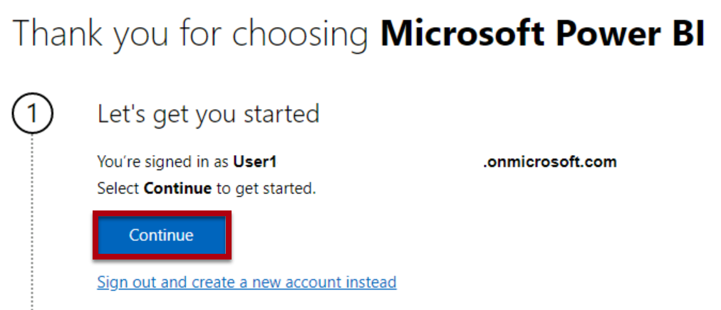
4. You will be redirected to the Power BI sign-up page in Microsoft Edge. Select Continue to complete the sign up.

   

5. Enter a 10 digit phone number and select Get started. Select Get started once more. You will be redirected to Power BI.

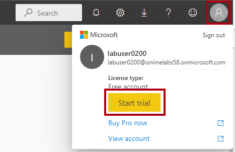
6. At the top-right, select the profile icon, and then select Start trial.

   

7. When prompted, select Start trial.

8. Do any remaining tasks to complete the trial setup.

   Tip: The Power BI web browser experience is known as the Power BI service.

Create a workspace in the Power BI Service

In this task, you will create a workspace.

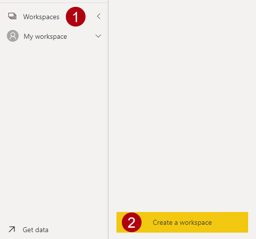
1. In the Power BI service, to create a workspace, in the Navigation pane (located at the left), select Workspaces, and then select Create workspace.

   

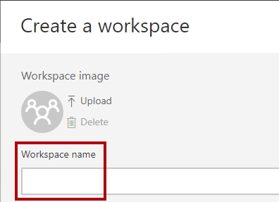
2. In the Create a workspace pane (located at the right), in the Workspace name box, enter a name for the workspace.

   The workspace name must be unique within the tenant.

   

3. Select Save.

   

   Once created, the workspace opens. In the next task, you will publish a dataset to this workspace.

Open the starter file in Power BI Desktop

1. To open File Explorer, on the taskbar, select the File Explorer shortcut.

2. Go to the D:\DP500\Allfiles\16\Starter folder.

3. To open a pre-developed Power BI Desktop file, double-click the Sales Analysis - Create reusable Power BI artifacts.pbix file.

4. If you’re not already signed in, at the top-right corner of Power BI Desktop, select Sign In. Use the lab credentials to complete the sign in process.

   

Review the data model

In this task, you will review the data model.

1. In Power BI Desktop, at the left, switch to Model view.

   

2. Use the model diagram to review the model design.

   

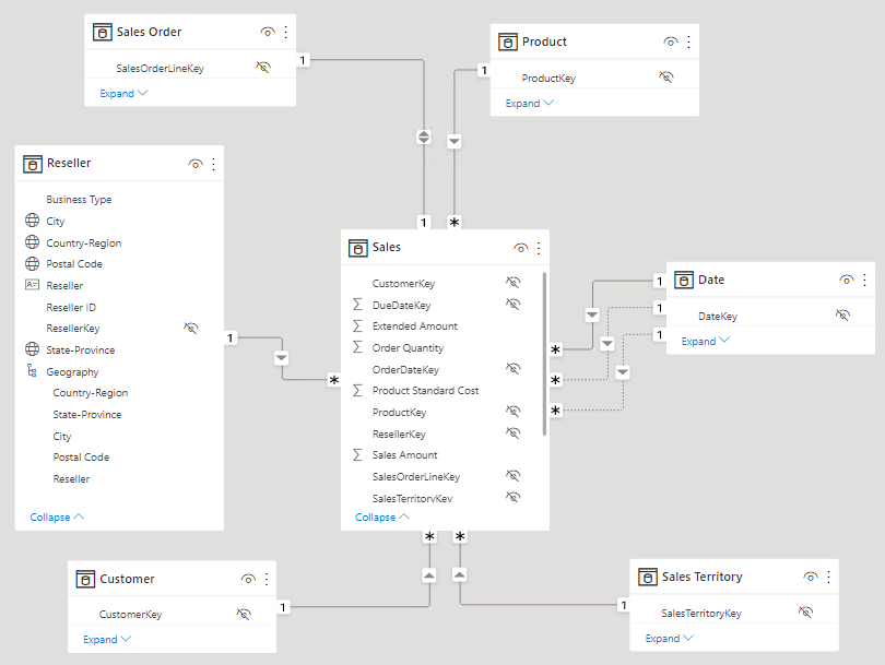
   The model comprises six dimension tables and one fact table. The Sales fact table stores sales order details. It’s a classic star schema design.

Publish the data model

In this task, you will publish the data model.

1. To publish the report, on the Home ribbon tab, select Publish.

   If prompted to save changes, select Save.

   

2. In the Publish to Power BI window, select your workspace (not the personal workspace), and then select Select.

3. When the publishing succeeds, select Got it.

   Once published, the model becomes a Power BI dataset. In this lab, this dataset is a core dataset that a business analyst can extend to create a specialized dataset. In the next exercise, you will create a specialized dataset to solve a specific business requirement.

4. Close Power BI Desktop.

5. If prompted to save changes, select Don’t save.

Create a specialized dataset

In this exercise, you will create a specialized dataset to allow the analysis of US sales per capita. Because the core dataset doesn’t contain population values, you will add a new table to extend the model.

Create a live connection

In this task, you will create a new report that uses a live connection to the Sales Analysis - Create reusable Power BI artifacts dataset, which you published in the previous exercise.

1. To open Power BI Desktop, on the taskbar, select the Power BI Desktop shortcut.

2. Close the getting started window.

3. To save the file, on the File ribbon, select Save as.

4. In the Save As window, go to the D:\DP500\Allfiles\16\MySolution folder.

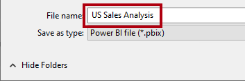
5. In the File name box, enter US Sales Analysis.

   

6. Select Save.

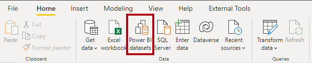
7. To create a live connection, on the Home ribbon tab, from inside the Data group, select Power BI datasets.

   

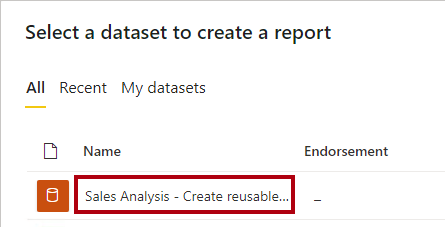
8. In the Data hub window, select the Sales Analysis - Create reusable Power BI artifacts dataset.

   

9. Select Connect.

10. In the Connect your data dialogue check the box next to Sales Analysis - Create reusable Power BI artifacts and then select Submit to connect to the data source.

11. When prompted about a potential security risk, read the notification, and then select OK.

12. At the bottom left, in the status bar, notice that the report connects live to the dataset.

    

13. Switch to Model view.

    

14. If necessary, to fit the model diagram to your screen, at the bottom right, select Fit to screen.

    

15. Hover the cursor over any table header to reveal a tooltip, and notice that the data source type is SQL Server Analysis Services, the server refers to your workspace, and the database is the dataset.

    

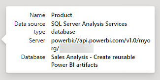
    These properties indicate that a remote model hosts the table. In the next task, you will make changes to the model to extend it. That process will create a local DirectQuery model that you can modify in many different ways.

16. Save the Power BI Desktop file.

    

Create a local DirectQuery model

In this task, you will create a local DirectQuery model.

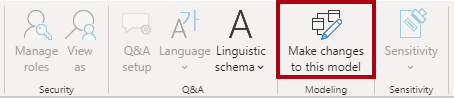
1. On the Home ribbon tab, from inside the Modeling group, select Make changes to this model.

   

   Note: if you do not see the option to make changes to this model, you need to enable the preview feature, DirectQuery for PBI datasets and AS

   • Navigate to File > Options and settings > Options, and in the Preview features section, select the DirectQuery for Power BI datasets and Analysis Services checkbox to enable this preview feature. You may need to restart Power BI Desktop for the change to take effect.

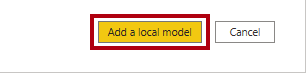
2. When prompted, read the dialog window message, and then select Add a local model.

   

   The model is now a DirectQuery model. It’s now possible to enhance the model by modifying certain table or column properties, or adding calculated columns. It’s even possible to extend the model with new tables of data that are sourced from other data sources. You will add a table to add US population data to the model.

3. In the Connect your data dialogue confirm you have a check in the box next to Sales Analysis - Create reusable Power BI artifacts and then select Submit to change the data source storage mode.

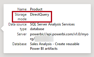
4. Hover the cursor over any table header to reveal a tooltip, and notice that the table storage mode is set to DirectQuery.

   

Design the report layout

In this task, you will design the report layout to analyze US state sales.

1. Switch to Report view.

   

2. In the Data pane (located at the right), expand open the Reseller table.

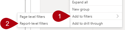
3. Right-click the Country-Region field, and then select Add to filters > Report-level filters.

   

4. Expand open the Filters pane (located at the left of the Visualizations pane).

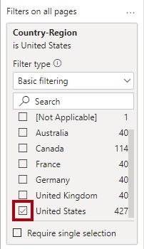
5. In the Filters pane, in the Filters on all pages section, in the Country-Region card, select United States.

   

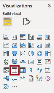
6. To add a table visual, in the Visualizations pane, select the table visual icon.

   

7. Reposition and resize the table so that it fills the entire page.

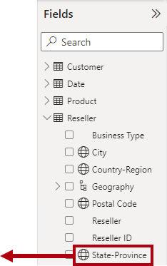
8. In the Data pane, from inside the Reseller table, drag the State-Province field and drop it into the table visual.

   

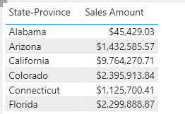
9. In the Data pane, expand the Sales table, and then add the Sales Amount field to the table visual.

   

10. To sort the states by descending order of sales amount, select the Sum of Sales Amount header.

    This report layout now provides basic detail about US state sales. However, an additional requirement is to show sales per capita and sort states by descending order of that measure.

Add a table

In this task, you will add a table of US population data sourced from a web page.

1. Switch to Model view.

   

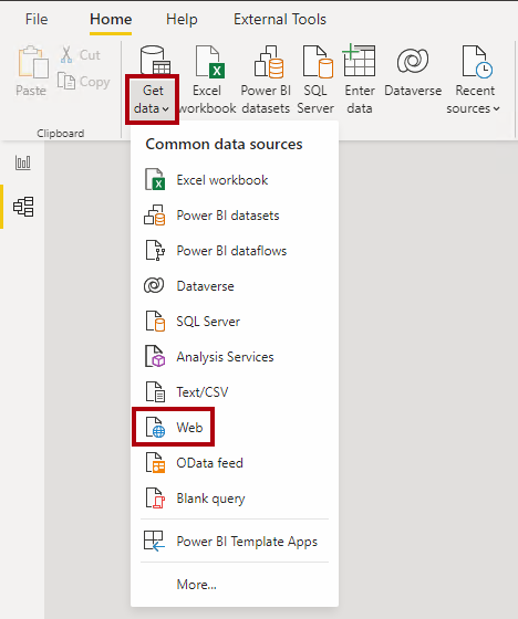
2. On the Home ribbon tab, from inside the Data group, select Get data, and then select Web.

   

3. In the URL box, enter the following file path: D:\DP500\Allfiles\16\Assets\us-resident-population-estimates-2020.html

   For the purposes of this lab, Power BI Desktop will access the web page from the file system.

   Tip: The file path is available to copy and paste from the D:\DP500\Allfiles\16\Assets\Snippets.txt file.

4. Select OK.

   

5. In the Navigator window, at the right, switch to Web View.

   

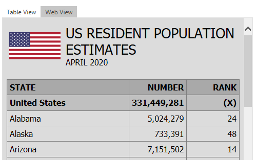
   The web page presents US resident population estimates sourced from the April 2020 census.

6. Switch back to Table view.

   

7. At the left, select Table 2.

   

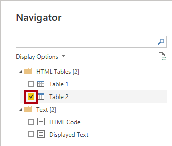
8. Notice the table view preview.

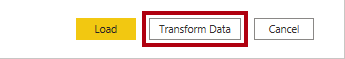
   This table of data contains the data that’s required by your model to calculate sales per capita. You will need to prepare the data by applying transformations: Specifically, you will remove the row for United States, remove the RANK column, and rename the STATE and NUMBER columns.

9. To prepare the data, select Transform Data.

   

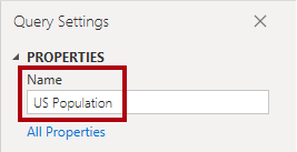
10. In the Power Query Editor window, in the Query Settings pane (located at the right), in the Name box, replace the text with US Population, and then press Enter.

    

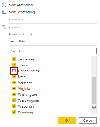
11. To remove the United States row, in the STATE column header, select the down-arrow, and then unselect the United States item (scroll to the bottom of the list).

    

12. Select OK.

    

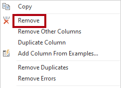
13. To remove the RANK column, right-click the column header, and then select Remove.

    

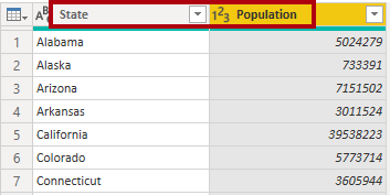
14. To rename the STATE column, double-click the column header, replace the text with State, and then press Enter.

15. Rename the NUMBER column as Population.

    

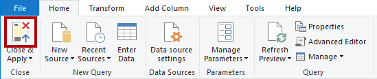
16. To apply the query, on the Home ribbon tab, from inside the Close group, select the Close & Apply icon.

    

17. When prompted about a potential security risk, read the notification, and then select OK.

    

    Power BI Desktop applies the query to create a model table. It adds a new table that imports population data to the model.

18. Reposition the US Population table near the Reseller table.

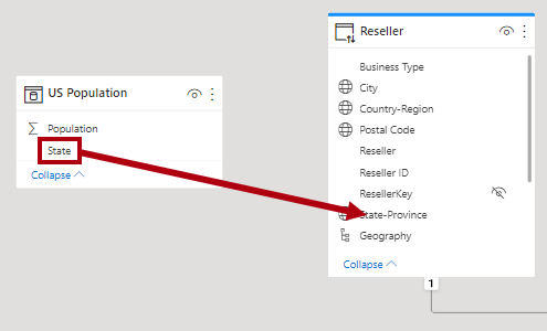
19. To create a model relationship, from the US Population table, drag the State column and drop it on the State-Province column of the Reseller table.

    

20. In the Create Relationship window, in the Cross Filter Direction dropdown list, select Both.

    

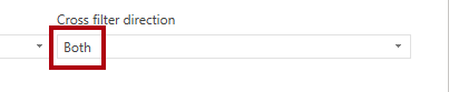
    Each row of the Reseller table stores a reseller, so the values found in the State-Province column will contain duplicate values (for example, there are many resellers in the state of California). When you create the relationship, Power BI Desktop automatically determines column cardinalities and discovered that it’s a many-to-one relationship. To ensure filters propagate from the Reseller table to the US Population table, the relationship must cross filter in both directions.

21. Select OK.

    

22. To hide the new table, in the header of the US Population table, select the visibility icon.

    

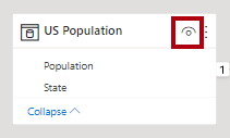
    The table doesn’t need to be visible to report authors.

Add a measure

In this task, you will add a measure to calculate sales per capita.

1. Switch to Report view.

   

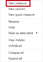
2. In the Data pane, right-click the Sales table, and then select New measure.

   

3. In the formula bar, enter the following measure definition.

   Tip: The measure definition is available to copy and paste from the D:\DP500\Allfiles\16\Assets\Snippets.txt file.

    Sales per Capita =
    DIVIDE(
    SUM(Sales[Sales Amount]),
    SUM('US Population'[Population])
    )
   

   The measure named Sales per Capita uses the DAX DIVIDE function to divide the sum of the Sales Amount column by the sum of the Population column.

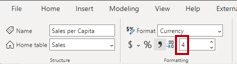
4. On the Measure Tools contextual ribbon tab, from inside the Formatting group, in the decimal places box, enter 4.

   

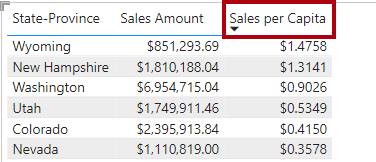
5. To add the measure to the matrix visual, in the Data pane, from inside the Sales table, drag the Sales per Capita field into the table visual.

   The measure evaluates the result by combining data sourced from a remote model in the Power BI service with data from the imported table that is local to your new model.

6. To sort the states by descending sales per capita value, select the Sales per Capita column header.

   

Publish the solution

In this task, you will publish the solution, which comprises a specialized data model and a report.

1. Save the Power BI Desktop file.

   

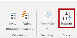
2. To publish the solution, on the Home ribbon tab, select Publish.

   

3. In the Publish to Power BI window, select your workspace, and then select Select.

   

4. When the publishing succeeds, select Got it.

   

5. Close Power BI Desktop.

6. If prompted to save changes, select Don’t save.

   

Review the specialized dataset

In this task, you will review the specialized dataset in the Power BI service.

1. Switch to the Power BI service (web browser).

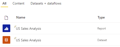
2. In the workspace landing page, notice the US Sales Analysis report and US Sales Analysis dataset.

   

3. Hover the cursor over the US Sales Analysis dataset, and when the ellipsis appears, select the ellipsis, and then select View lineage.

   

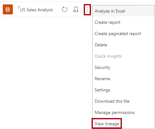
   The View lineage option supports finding out dependencies between Power BI assets. That’s important, for example, if you are going to publish changes to a core dataset. Lineage view will tell you the dependent datasets that might require testing.

4. In lineage view, notice the connection between the report, the US Sales Analysis dataset, and the Sales Analysis - Create reusable Power BI artifacts dataset.

   

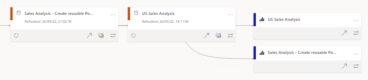
   When Power BI datasets relate to other datasets, it’s known as chaining. In this lab, the US Sales Analysis dataset is chained to the Sales Analysis - Create reusable Power BI artifacts dataset, enabling its reuse for a specialized purpose.