Create a composite model

Overview

The estimated time to complete the lab is 30 minutes.

In this lab, you will create a composite model by adding a table to a pre-developed DirectQuery model.

In this lab, you learn how to:

Create a composite model.
Create model relationships.
Create measures.

Get started

In this exercise, you will prepare your environment.

Clone the repository for this course

On the start menu, open the Command Prompt
In the command prompt window, navigate to the D drive by typing:

d:

Press enter.
In the command prompt window, enter the following command to download the course files and save them to a folder called DP500.

git clone https://github.com/MicrosoftLearning/DP-500-Azure-Data-Analyst DP500
When the repository has been cloned, close the command prompt window.
Open the D drive in the file explorer to ensure the files have been downloaded.

Set up Power BI Desktop

In this task, you will open a pre-developed Power BI template file.

To open File Explorer, on the taskbar, select the File Explorer shortcut.
Go to the D:\DP500\Allfiles\08\Starter folder.
To open a pre-developed Power BI Desktop file, double-click the Sales Analysis - Create a composite model.pbit file.
If prompted to approve a potential security risk, select OK.
Enter the SQLServerInstance, SqlServerDatabase, and Culture as provided below. Select Load.

SqlServerInstance = localhost

SqlServerDatabase = AdventureWorksDW2022-DP500

Culture = en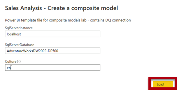
In the SQL server database connection prompt, select Connect.
In the Encryption Support window, select OK.
In the Native Database Query window, select Run.
Save the file. On the File menu, select Save as.
In the Save As window, go to the D:\DP500\Allfiles\08\MySolution folder. The file name is Sales Analysis - Create a composite model.pbix.
Select Save.

Review the report

In this task, you will review the pre-developed report.

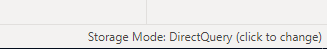
In Power BI Desktop, at the bottom right corner in the status bar, notice that the storage mode is DirectQuery.

A DirectQuery model comprises tables that use DirectQuery storage mode. A table that uses DirectQuery storage mode passes queries through to the underlying data source. Data modelers often use this storage mode to model large volumes of data. In this instance, the underlying data source is a SQL Server database.
Review the report design.

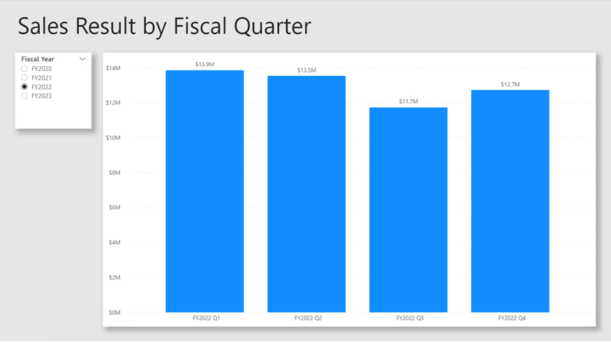
This report page has a title and two visuals. The slicer visual allows filtering by a single fiscal year, while the column chart visual displays quarterly sales amounts. You will improve upon this design by adding sales targets to the column chart visual.
In the Fiscal Year slicer, select FY2021.

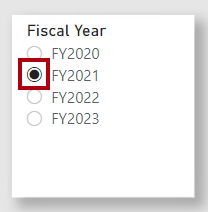
It’s important to understand that slicer selections change the filters applied to the column chart visual. Power BI refreshes the column chart visual. That involves retrieving data from the source database. That way, the column chart visual shows the latest source data. (Some report-level caching may occur, meaning the report may reuse previously queried data.)

Review the data model

In this task, you will review the pre-developed data model.

Switch to Model view.
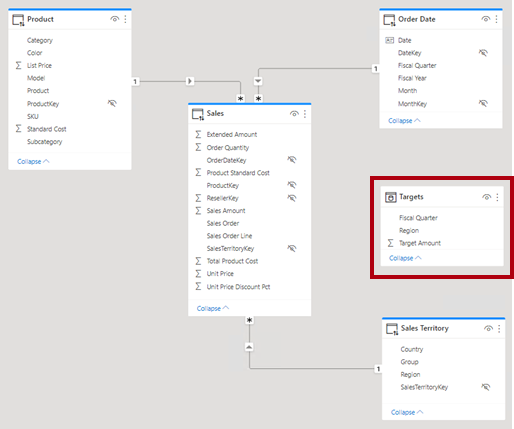
Use the model diagram to review the model design.

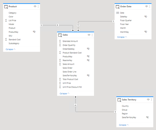
The model comprises three dimension tables and one fact table. The Sales fact table represents sales order details. It’s a classic star schema design. The bar across the top of each table indicates it uses DirectQuery storage mode. Because each table has a blue bar, it indicates all tables belong to the same source group.

You will extend the model with another fact table to support analyzing sales target facts too.

Create a composite model

In this exercise, you will add an import table that will convert the DirectQuery model to a composite model.

A composite model comprises more than one source group.

Add a table

In this task, you will add a table that stores sales targets sourced from an Excel workbook.

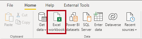
On the Home ribbon tab, from inside the Data group, select Excel workbook.
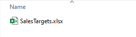
In the Open window, go to the D:\DP500\Allfiles\08\Assets folder.
Select the SalesTargets.xlsx file.
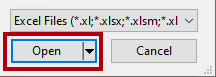
Select Open.
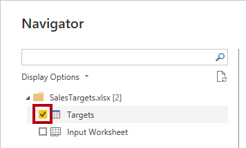
In the Navigator window, check the Targets table.
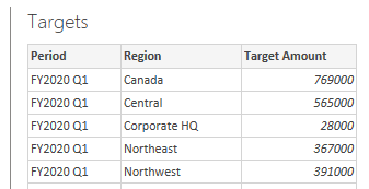
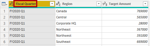
In the preview pane (located at the right), notice that the table comprises three columns, and each row of the table represents a fiscal quarter, sales region, and a target sales amount.

You will import this data to add a table to the DirectQuery model. Because it isn’t possible to connect to an Excel workbook using DirectQuery, Power BI will import it.
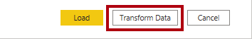
Select Transform Data.
In the Power Query Editor window, to rename the first column, double-click the Period column header.
Rename the column as Fiscal Quarter, and then press Enter.
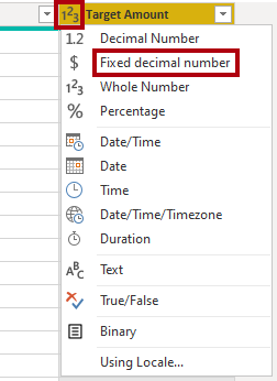
To modify the data type of the third column, in the Target Amount column header, select the data type icon (123), and then select Fixed Decimal Number.
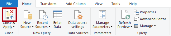
To apply the query, on the Home ribbon tab, from inside the Close group, select the Close & Apply icon.
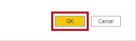
If prompted about a potential security risk, read the message, and then select OK.
In Power BI Desktop, when the load process completes, in the model diagram, position the new table directly beneath the Order Date table.

The table may be out of view. If this is the case, scroll horizontally to reveal the table.
Notice that the Targets table doesn’t have a blue bar across the top.

The absence of a bar indicates the table belongs to the import source group.

Create model relationships

In this task, you will create two model relationships.

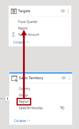
To create a relationship, from the Sales Territory table, drag the Region column and drop it on to the Region column of the Targets table.
In the Create relationship window, notice that the Cardinality dropdown list is set to One to many.

The Region column in the Sales Territory table contains unique values, while the Region column in the Targets table contains duplicate values. This one-to-many cardinality is common for relationships between dimension and fact tables.
Select OK.
In the model diagram, notice that a relationship now exists between the Sales Territory and Target tables.
Notice also that the relationship line look different to the other relationship lines.

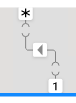
The “disconnected” line indicates that the relationship is a limited relationship. A model relationship is limited when there’s no guaranteed “one” side. In this case, it’s because the relationship spans source groups. At query time, relationship evaluation can differ for limited relationships. For more information, see Limited relationships.
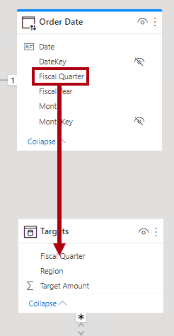
Create another relationship, this time relating the Fiscal Quarter column of the Order Date table to the Fiscal Quarter column of the Targets table.
In the Create relationship window, notice that the Cardinality dropdown list is set to Many to many.

Because both columns contain duplicate values, Power BI Desktop automatically sets the cardinality to many to many. However, the default cross filter direction is incorrect.
In the Cross filter direction dropdown list, select Single (Order Date filters Targets).

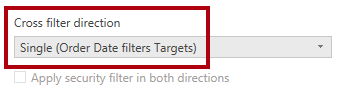
It’s common that dimension tables filter fact tables. In this model design, it isn’t necessary (or efficient) to propagate filters from the fact table to the dimension table.
Select OK.

Set model properties

In this task, you will set model properties of the new table.

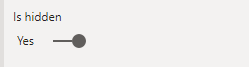
In the Targets table, select the Fiscal Quarter column.
While pressing the Ctrl key, also select the Region column.
In the Properties pane, set the Is hidden property to Yes.
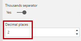
In the Targets table, select the Target Amount column.
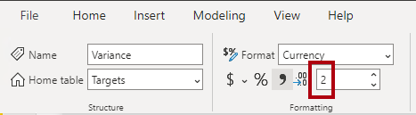
In the Properties pane, in the Formatting section, set the Decimal places property to 2.

Add measures

In this task, you will add two measures to allow the analysis of sales target variance.

Switch to Report view.
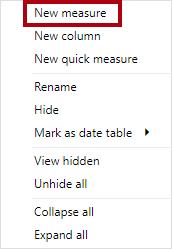
To create a measure, in the Data pane (located at the right), right-click the Targets table, and then select New measure.
In the formula bar, enter the following measure definition.

Tip: All measure definitions are available to copy and paste from the D:\DP500\Allfiles\08\Assets\Snippets.txt file.
```
 Variance = SUM ( 'Sales'[Sales Amount] ) - SUM ( 'Targets'[Target Amount] )
```
The measure named Variance subtracts the sum of Target Amount from the sum of Sales Amount.
On the Measure Tools contextual ribbon tab, from inside the Formatting group, in the decimal places box, enter 2.
Create another measure using the following measure definition.
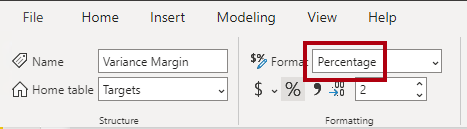
```
 Variance Margin =

 DIVIDE (

 [Variance],

 SUM ( 'Targets'[Target Amount] )

 )
```
The measure named Variance Margin uses the DAX DIVIDE function to divide the Variance measure by the sum of the Target Amount column.
On the Measure Tools contextual ribbon tab, from inside the Formatting group, in the Format dropdown list, select Percentage.
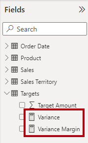
In the Data pane, inside the Targets table, verify that there are two measures.

Update the report layout

In this task, you will update the report to use the new measures.

In the report, select the column chart visual.
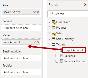
From the Data pane, drag the Target Amount field into the Visualizations pane, inside the Values well, directly beneath the Sales Amount field.
Notice that the column chart visual now shows sales and target amounts.
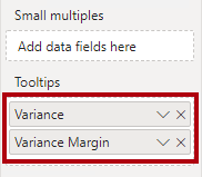
Drag the two measures into the Tooltips well.
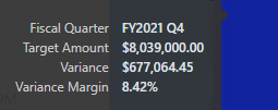
Hover the cursor over any column to reveal a tooltip, and notice that it shows the measure values.

You have now completed the creation of a composite model that combines DirectQuery and import tables. You could optimize the model to improve query performance by setting dimension tables to use dual storage mode, and by adding aggregations. However, those enhancements will be the learning objective of other labs.

Finish up

In this task, you will finish up.

Save the Power BI Desktop file.
Close Power BI Desktop.