Explore a relational data warehouse

Azure Synapse Analytics is built on a scalable set capabilities to support enterprise data warehousing; including file-based data analytics in a data lake as well as large-scale relational data warehouses and the data transfer and transformation pipelines used to load them. In this lab, you’ll explore how to use a dedicated SQL pool in Azure Synapse Analytics to store and query data in a relational data warehouse.

This lab will take approximately 45 minutes to complete.

Before you start

You’ll need an Azure subscription in which you have administrative-level access.

Provision an Azure Synapse Analytics workspace

An Azure Synapse Analytics workspace provides a central point for managing data and data processing runtimes. You can provision a workspace using the interactive interface in the Azure portal, or you can deploy a workspace and resources within it by using a script or template. In most production scenarios, it’s best to automate provisioning with scripts and templates so that you can incorporate resource deployment into a repeatable development and operations (DevOps) process.

In this exercise, you’ll use a combination of a PowerShell script and an ARM template to provision Azure Synapse Analytics.

Sign into the Azure portal at https://portal.azure.com.
Use the [>_] button to the right of the search bar at the top of the page to create a new Cloud Shell in the Azure portal, selecting a PowerShell environment and creating storage if prompted. The cloud shell provides a command line interface in a pane at the bottom of the Azure portal, as shown here:

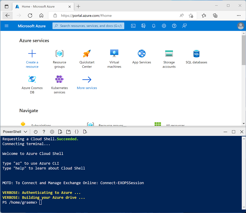
Note: If you have previously created a cloud shell that uses a Bash environment, use the the drop-down menu at the top left of the cloud shell pane to change it to PowerShell.
Note that you can resize the cloud shell by dragging the separator bar at the top of the pane, or by using the —, ◻, and X icons at the top right of the pane to minimize, maximize, and close the pane. For more information about using the Azure Cloud Shell, see the Azure Cloud Shell documentation.

In the PowerShell pane, enter the following commands to clone this repo:

 rm -r dp500 -f
 git clone https://github.com/MicrosoftLearning/DP-500-Azure-Data-Analyst dp500

After the repo has been cloned, enter the following commands to change to the folder for this lab and run the setup.ps1 script it contains:
```
 cd dp500/Allfiles/03
 ./setup.ps1
```
If prompted, choose which subscription you want to use (this will only happen if you have access to multiple Azure subscriptions).
When prompted, enter a suitable password to be set for your Azure Synapse SQL pool.

Note: Be sure to remember this password!
Wait for the script to complete - this typically takes around 15 minutes, but in some cases may take longer. While you are waiting, review the What is dedicated SQL pool in Azure Synapse Analytics? article in the Azure Synapse Analytics documentation.

Explore the data warehouse schema

In this lab, the data warehouse is hosted in a dedicated SQL pool in Azure Synapse Analytics.

Start the dedicated SQL pool

After the script has completed, in the Azure portal, go to the dp500-xxxxxxx resource group that it created, and select your Synapse workspace.
In the Overview page for your Synapse workspace, in the Open Synapse Studio card, select Open to open Synapse Studio in a new browser tab; signing in if prompted.
On the left side of Synapse Studio, use the ›› icon to expand the menu - this reveals the different pages within Synapse Studio that are used to manage resources and perform data analytics tasks.
On the Manage page, ensure the SQL pools tab is selected and then select the sqlxxxxxxx dedicated SQL pool and use its ▷ icon to start it; confirming that you want to resume it when prompted.
Wait for the SQL pool to resume. This can take a few minutes. Use the ↻ Refresh button to check its status periodically. The status will show as Online when it is ready.

View the tables in the database

In Synapse Studio, select the Data page and ensure that the Workspace tab is selected and contains a SQL database category.
Expand SQL database, the sqlxxxxxxx pool, and its Tables folder to see the tables in the database.

A relational data warehouse is typically based on a schema that consists of fact and dimension tables. The tables are optimized for analytical queries in which numeric metrics in the fact tables are aggregated by attributes of the entities represented by the dimension tables - for example, enabling you to aggregate Internet sales revenue by product, customer, date, and so on.
Expand the dbo.FactInternetSales table and its Columns folder to see the columns in this table. Note that many of the columns are keys that reference rows in the dimension tables. Others are numeric values (measures) for analysis.

The keys are used to relate a fact table to one or more dimension tables, often in a star schema; in which the fact table is directly related to each dimension table (forming a multi-pointed “star” with the fact table at the center).
View the columns for the dbo.DimPromotion table, and note that it has a unique PromotionKey that uniquely identifies each row in the table. It also has an AlternateKey.

Usually, data in a data warehouse has been imported from one or more transactional sources. The alternate key reflects the business identifier for the instance of this entity in the source, but a unique numeric surrogate key is usually generated to uniquely identify each row in the data warehouse dimension table. One of the benefits of this approach is that it enables the data warehouse to contain multiple instances of the same entity at different points in time (for example, records for the same customer reflecting their address at the time an order was placed).
View the columns for the dbo.DimProduct, and note that it contains a ProductSubcategoryKey column, which references the dbo.DimProductSubcategory table, which in turn contains a ProductCategoryKey column that references the dbo.DimProductCategory table.

In some cases, dimensions are partially normalized into multiple related tables to allow for different levels of granularity - such as products that can be grouped into subcategories and categories. This results in a simple star being extended to a snowflake schema, in which the central fact table is related to a dimension table, which is turn related to further dimension tables.
View the columns for the dbo.DimDate table, and note that it contains multiple columns that reflect different temporal attributes of a date - including the day of week, day of month, month, year, day name, month name, and so on.

Time dimensions in a data warehouse are usually implemented as a dimension table containing a row for each of the smallest temporal units of granularity (often called the grain of the dimension) by which you want to aggregate the measures in the fact tables. In this case, the lowest grain at which measures can be aggregated is an individual date, and the table contains a row for each date from the first to the last date referenced in the data. The attributes in the DimDate table enable analysts to aggregate measures based on any date key in the fact table, using a consistent set of temporal attributes (for example, viewing orders by month based on the order date). The FactInternetSales table contains three keys that relate to the DimDate table: OrderDateKey, DueDateKey, and ShipDateKey.

Query the data warehouse tables

Now that you have explored some of the more important aspects of the data warehouse schema, you’re ready to to query the tables and retrieve some data.

Query fact and dimension tables

Numeric values in a relational data warehouse are stored in fact tables with related dimension tables that you can use to aggregate the data across multiple attributes. This design means that most queries in a relational data warehouse involve aggregating and grouping data (using aggregate functions and GROUP BY clauses) across related tables (using JOIN clauses).

On the Data page, select the sqlxxxxxxx SQL pool and in its … menu, select New SQL script > Empty script.
When a new SQL Script 1 tab opens, in its Properties pane, change the name of the script to Analyze Internet Sales and change the Result settings per query to return all rows. Then use the Publish button on the toolbar to save the script, and use the Properties button (which looks similar to 🗏.) on the right end of the toolbar to close the Properties pane so you can see the script pane.

In the empty script, add the following code:

 SELECT  d.CalendarYear AS Year,
         SUM(i.SalesAmount) AS InternetSalesAmount
 FROM FactInternetSales AS i
 JOIN DimDate AS d ON i.OrderDateKey = d.DateKey
 GROUP BY d.CalendarYear
 ORDER BY Year;

Use the ▷ Run button to run the script, and review the results, which should show the Internet sales totals for each year. This query joins the fact table for Internet sales to a time dimension table based on the order date, and aggregates the sales amount measure in the fact table by the calendar month attribute of the dimension table.
Modify the query as follows to add the month attribute from the time dimension, and then run the modified query.
```
 SELECT  d.CalendarYear AS Year,
         d.MonthNumberOfYear AS Month,
         SUM(i.SalesAmount) AS InternetSalesAmount
 FROM FactInternetSales AS i
 JOIN DimDate AS d ON i.OrderDateKey = d.DateKey
 GROUP BY d.CalendarYear, d.MonthNumberOfYear
 ORDER BY Year, Month;
```
Note that the attributes in the time dimension enable you to aggregate the measures in the fact table at multiple hierarchical levels - in this case, year and month. This is a common pattern in data warehouses.

Modify the query as follows to remove the month and add a second dimension to the aggregation, and then run it to view the results (which show yearly Internet sales totals for each region):

 SELECT  d.CalendarYear AS Year,
         g.EnglishCountryRegionName AS Region,
         SUM(i.SalesAmount) AS InternetSalesAmount
 FROM FactInternetSales AS i
 JOIN DimDate AS d ON i.OrderDateKey = d.DateKey
 JOIN DimCustomer AS c ON i.CustomerKey = c.CustomerKey
 JOIN DimGeography AS g ON c.GeographyKey = g.GeographyKey
 GROUP BY d.CalendarYear, g.EnglishCountryRegionName
 ORDER BY Year, Region;

Note that geography is a snowflake dimension that is related to the Internet sales fact table through the customer dimension. You therefore need two joins in the query to aggregate Internet sales by geography.

Modify and re-run the query to add another snowflake dimension and aggregate the yearly regional sales by product category:

 SELECT  d.CalendarYear AS Year,
         pc.EnglishProductCategoryName AS ProductCategory,
         g.EnglishCountryRegionName AS Region,
         SUM(i.SalesAmount) AS InternetSalesAmount
 FROM FactInternetSales AS i
 JOIN DimDate AS d ON i.OrderDateKey = d.DateKey
 JOIN DimCustomer AS c ON i.CustomerKey = c.CustomerKey
 JOIN DimGeography AS g ON c.GeographyKey = g.GeographyKey
 JOIN DimProduct AS p ON i.ProductKey = p.ProductKey
 JOIN DimProductSubcategory AS ps ON p.ProductSubcategoryKey = ps.ProductSubcategoryKey
 JOIN DimProductCategory AS pc ON ps.ProductCategoryKey = pc.ProductCategoryKey
 GROUP BY d.CalendarYear, pc.EnglishProductCategoryName, g.EnglishCountryRegionName
 ORDER BY Year, ProductCategory, Region;

This time, the snowflake dimension for product category requires three joins to reflect the hierarchical relationship between products, subcategories, and categories.

Publish the script to save it.

Use ranking functions

Another common requirement when analyzing large volumes of data is to group the data by partitions and determine the rank of each entity in the partition based on a specific metric.

Under the existing query, add the following SQL to retrieve sales values for 2022 over partitions based on country/region name:

 SELECT  g.EnglishCountryRegionName AS Region,
         ROW_NUMBER() OVER(PARTITION BY g.EnglishCountryRegionName
                           ORDER BY i.SalesAmount ASC) AS RowNumber,
         i.SalesOrderNumber AS OrderNo,
         i.SalesOrderLineNumber AS LineItem,
         i.SalesAmount AS SalesAmount,
         SUM(i.SalesAmount) OVER(PARTITION BY g.EnglishCountryRegionName) AS RegionTotal,
         AVG(i.SalesAmount) OVER(PARTITION BY g.EnglishCountryRegionName) AS RegionAverage
 FROM FactInternetSales AS i
 JOIN DimDate AS d ON i.OrderDateKey = d.DateKey
 JOIN DimCustomer AS c ON i.CustomerKey = c.CustomerKey
 JOIN DimGeography AS g ON c.GeographyKey = g.GeographyKey
 WHERE d.CalendarYear = 2022
 ORDER BY Region;

Select only the new query code, and use the ▷ Run button to run it. Then review the results, which should look similar to the following table:

Region	RowNumber	OrderNo	LineItem	SalesAmount	RegionTotal	RegionAverage
Australia	1	SO73943	2	2.2900	2172278.7900	375.8918
Australia	2	SO74100	4	2.2900	2172278.7900	375.8918
…	…	…	…	…	…	…
Australia	5779	SO64284	1	2443.3500	2172278.7900	375.8918
Canada	1	SO66332	2	2.2900	563177.1000	157.8411
Canada	2	SO68234	2	2.2900	563177.1000	157.8411
…	…	…	…	…	…	…
Canada	3568	SO70911	1	2443.3500	563177.1000	157.8411
France	1	SO68226	3	2.2900	816259.4300	315.4016
France	2	SO63460	2	2.2900	816259.4300	315.4016
…	…	…	…	…	…	…
France	2588	SO69100	1	2443.3500	816259.4300	315.4016
Germany	1	SO70829	3	2.2900	922368.2100	352.4525
Germany	2	SO71651	2	2.2900	922368.2100	352.4525
…	…	…	…	…	…	…
Germany	2617	SO67908	1	2443.3500	922368.2100	352.4525
United Kingdom	1	SO66124	3	2.2900	1051560.1000	341.7484
United Kingdom	2	SO67823	3	2.2900	1051560.1000	341.7484
…	…	…	…	…	…	…
United Kingdom	3077	SO71568	1	2443.3500	1051560.1000	341.7484
United States	1	SO74796	2	2.2900	2905011.1600	289.0270
United States	2	SO65114	2	2.2900	2905011.1600	289.0270
…	…	…	…	…	…	…
United States	10051	SO66863	1	2443.3500	2905011.1600	289.0270

Observe the following facts about these results:

There’s a row for each sales order line item.
The rows are organized in partitions based on the geography where the sale was made.
The rows within each geographical partition are numbered in order of sales amount (from smallest to highest).
For each row, the line item sales amount as well as the regional total and average sales amounts are included.

Under the existing queries, add the following code to apply windowing functions within a GROUP BY query and rank the cities in each region based on their total sales amount:

 SELECT  g.EnglishCountryRegionName AS Region,
         g.City,
         SUM(i.SalesAmount) AS CityTotal,
         SUM(SUM(i.SalesAmount)) OVER(PARTITION BY g.EnglishCountryRegionName) AS RegionTotal,
         RANK() OVER(PARTITION BY g.EnglishCountryRegionName
                     ORDER BY SUM(i.SalesAmount) DESC) AS RegionalRank
 FROM FactInternetSales AS i
 JOIN DimDate AS d ON i.OrderDateKey = d.DateKey
 JOIN DimCustomer AS c ON i.CustomerKey = c.CustomerKey
 JOIN DimGeography AS g ON c.GeographyKey = g.GeographyKey
 GROUP BY g.EnglishCountryRegionName, g.City
 ORDER BY Region;

Select only the new query code, and use the ▷ Run button to run it. Then review the results, and observe the following:
- The results include a row for each city, grouped by region.
- The total sales (sum of individual sales amounts) is calculated for each city
- The regional sales total (the sum of the sum of sales amounts for each city in the region) is calculated based on the regional partition.
- The rank for each city within its regional partition is calculated by ordering the total sales amount per city in descending order.
Publish the updated script to save the changes.

Tip: ROW_NUMBER and RANK are examples of ranking functions available in Transact-SQL. For more details, see the Ranking Functions reference in the Transact-SQL language documentation.

Retrieve an approximate count

When exploring very large volumes of data, queries can take significant time and resources to run. Often, data analysis doesn’t require absolutely precise values - a comparison of approximate values may be sufficient.

Under the existing queries, add the following code to retrieve the number of sales orders for each calendar year:

 SELECT d.CalendarYear AS CalendarYear,
     COUNT(DISTINCT i.SalesOrderNumber) AS Orders
 FROM FactInternetSales AS i
 JOIN DimDate AS d ON i.OrderDateKey = d.DateKey
 GROUP BY d.CalendarYear
 ORDER BY CalendarYear;

Select only the new query code, and use the ▷ Run button to run it. Then review the output that is returned:
- On the Results tab under the query, view the order counts for each year.
- On the Messages tab, view the total execution time for the query.

Modify the query as follows, to return an approximate count for each year. Then re-run the query.

 SELECT d.CalendarYear AS CalendarYear,
     APPROX_COUNT_DISTINCT(i.SalesOrderNumber) AS Orders
 FROM FactInternetSales AS i
 JOIN DimDate AS d ON i.OrderDateKey = d.DateKey
 GROUP BY d.CalendarYear
 ORDER BY CalendarYear;

Review the output that is returned:
- On the Results tab under the query, view the order counts for each year. These should be within 2% of the actual counts retrieved by the previous query.
- On the Messages tab, view the total execution time for the query. This should be shorter than for the previous query.
Publish the script to save the changes.

Tip: See the APPROX_COUNT_DISTINCT function documentation for more details.

Challenge - Analyze reseller sales

Create a new empty script for the sqlxxxxxxx SQL pool, and save it with the name Analyze Reseller Sales.
Create SQL queries in the script to find the following information based on the FactResellerSales fact table and the dimension tables to which it is related:
- The total quantity of items sold per fiscal year and quarter.
- The total quantity of items sold per fiscal year, quarter, and sales territory region associated with the employee who made the sale.
- The total quantity of items sold per fiscal year, quarter, and sales territory region by product category.
- The rank of each sales territory per fiscal year based on total sales amount for the year.
- The approximate number of sales order per year in each sales territory.
Tip: Compare your queries to the ones in the Solution script in the Develop page in Synapse Studio.
Experiment with queries to explore the rest of the tables in the data warehouse schema as your leisure.
When you’re done, on the Manage page, pause the sqlxxxxxxx dedicated SQL pool.

Delete Azure resources

If you’ve finished exploring Azure Synapse Analytics, you should delete the resources you’ve created to avoid unnecessary Azure costs.

Close the Synapse Studio browser tab and return to the Azure portal.
On the Azure portal, on the Home page, select Resource groups.
Select the dp500-xxxxxxx resource group for your Synapse Analytics workspace (not the managed resource group), and verify that it contains the Synapse workspace, storage account, and dedicated SQL pool for your workspace.
At the top of the Overview page for your resource group, select Delete resource group.
Enter the dp500-xxxxxxx resource group name to confirm you want to delete it, and select Delete.

After a few minutes, your Azure Synapse workspace resource group and the managed workspace resource group associated with it will be deleted.