Explore classification with Azure Machine Learning Designer

Note To complete this lab, you will need an Azure subscription in which you have administrative access.

Create an Azure Machine Learning workspace

Sign into the Azure portal using your Microsoft credentials.
Select + Create a resource, search for Machine Learning, and create a new Azure Machine Learning resource with an Azure Machine Learning plan. Use the following settings:
- Subscription: Your Azure subscription.
- Resource group: Create or select a resource group.
- Workspace name: Enter a unique name for your workspace.
- Region: Select the closest geographical region.
- Storage account: Note the default new storage account that will be created for your workspace.
- Key vault: Note the default new key vault that will be created for your workspace.
- Application insights: Note the default new application insights resource that will be created for your workspace.
- Container registry: None (one will be created automatically the first time you deploy a model to a container)
Select Review + create, then select Create. Wait for your workspace to be created (it can take a few minutes), and then go to the deployed resource.
Select Launch studio (or open a new browser tab and navigate to https://ml.azure.com, and sign into Azure Machine Learning studio using your Microsoft account).
In Azure Machine Learning studio, you should see your newly created workspace. If that is not the case, select your Azure directory in the left-hand menu. Then from the new left-hand menu select Workspaces, where all the workspaces associated to your directory are listed, and select the one you created for this exercise.

Note This module is one of many that make use of an Azure Machine Learning workspace, including the other modules in the Microsoft Azure AI Fundamentals: Explore visual tools for machine learning learning path. If you are using your own Azure subscription, you may consider creating the workspace once and reusing it in other modules. Your Azure subscription will be charged a small amount for data storage as long as the Azure Machine Learning workspace exists in your subscription, so we recommend you delete the Azure Machine Learning workspace when it is no longer required.

Create compute

In Azure Machine Learning studio, select the ≡ icon (a menu icon that looks like a stack of three lines) at the top left to view the various pages in the interface (you may need to maximize the size of your screen). You can use these pages in the left hand pane to manage the resources in your workspace. Select the Compute page (under Manage).
On the Compute page, select the Compute clusters tab, and add a new compute cluster with the following settings. You’ll use this to train a machine learning model:
- Location: Select the same as your workspace. If that location is not listed, choose the one closest to you.
- Virtual machine tier: Dedicated
- Virtual machine type: CPU
- Virtual machine size:
  - Choose Select from all options
  - Search for and select Standard_DS11_v2
- Select Next
- Compute name: enter a unique name.
- Minimum number of nodes: 0
- Maximum number of nodes: 2
- Idle seconds before scale down: 120
- Enable SSH access: Clear
- Select Create

Note Compute instances and clusters are based on standard Azure virtual machine images. For this module, the Standard_DS11_v2 image is recommended to achieve the optimal balance of cost and performance. If your subscription has a quota that does not include this image, choose an alternative image; but bear in mind that a larger image may incur higher cost and a smaller image may not be sufficient to complete the tasks. Alternatively, ask your Azure administrator to extend your quota.

The compute cluster will take some time to be created. You can move onto the next step while you wait.

Create a dataset

In Azure Machine Learning studio, expand the left pane by selecting the menu icon at the top left of the screen. Select the Data page (under Assets). The Data page contains specific data files or tables that you plan to work with in Azure ML. You can create datasets from this page as well.
On the Data page, under the Data assets tab, select + Create. Then configure a data asset with the following settings:
- Data type:
  - Name: diabetes-data
  - Description: Diabetes data
  - Dataset type: Tabular
- Data source: From web files
- Web URL:
  - Web URL: https://aka.ms/diabetes-data
  - Skip data validation: do not select
- Settings:
  - File format: Delimited
  - Delimiter: Comma
  - Encoding: UTF-8
  - Column headers: Only first file has headers
  - Skip rows: None
  - Dataset contains multi-line data: do not select
- Schema:
  - Include all columns other than Path
  - Review the automatically detected types
- Review
  - Select Create
After the dataset has been created, open it and view the Explore page to see a sample of the data. This data represents details from patients who have been tested for diabetes.

Create a pipeline in Designer and load data to canvas

To get started with Azure Machine Learning designer, first you must create a pipeline and add the dataset you want to work with.

In Azure Machine Learning studio, on the left pane select the Designer item (under Authoring), and then select + to create a new pipeline.
Change the draft name from Pipeline-Created-on-date to Diabetes Training.
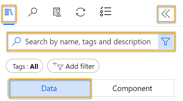
Then in the project, next to the pipeline name on the left, select the arrows icon to expand the panel if it is not already expanded. The panel should open by default to the Asset library pane, indicated by the books icon at the top of the panel. Note that there is a search bar to locate assets. Notice two buttons, Data and Component.
Select Data. Search for and place the diabetes-data dataset onto the canvas.
Right-click (Ctrl+click on a Mac) the diabetes-data dataset on the canvas, and select Preview data.
Review the schema of the data in the Profile tab, noting that you can see the distributions of the various columns as histograms.
Scroll down and select the column heading for the Diabetic column, and note that it contains two values 0 and 1. These values represent the two possible classes for the label that your model will predict, with a value of 0 meaning that the patient does not have diabetes, and a value of 1 meaning that the patient is diabetic.
Scroll back up and review the other columns, which represent the features that will be used to predict the label. Note that most of these columns are numeric, but each feature is on its own scale. For example, Age values range from 21 to 77, while DiabetesPedigree values range from 0.078 to 2.3016. When training a machine learning model, it is sometimes possible for larger values to dominate the resulting predictive function, reducing the influence of features that on a smaller scale. Typically, data scientists mitigate this possible bias by normalizing the numeric columns so they’re on the similar scales.
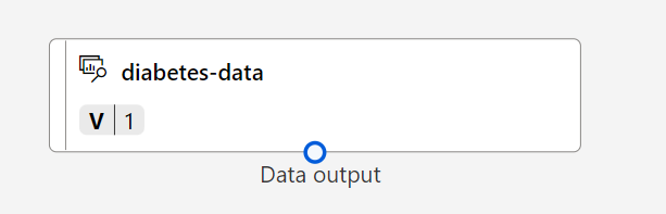
Close the DataOutput tab so that you can see the dataset on the canvas like this:

Add transformations

Before you can train a model, you typically need to apply some pre-processing transformations to the data.

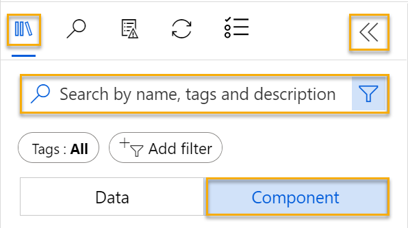
In the Asset library pane on the left, select Component, which contains a wide range of modules you can use for data transformation and model training. You can also use the search bar to quickly locate modules.
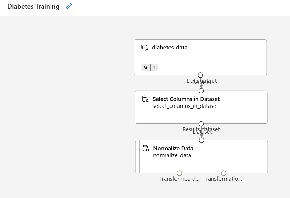
Find the Select Columns in Dataset module and place it on the canvas below the diabetes-data dataset. Then connect the output from the bottom of the diabetes-data dataset to the input at the top of the Select Columns in Dataset module.
Double click on the Select Columns in Dataset module to access a settings pane on the right. Select Edit column. Then in the Select columns window, select By name and Add all the columns. Then remove PatientID and click Save.
Find the Normalize Data module and place it on the canvas below the Select Columns in Dataset module. Then connect the output from the bottom of the Select Columns in Dataset module to the input at the top of the Normalize Data module, like this:
Double-click the Normalize Data module to view its settings, noting that it requires you to specify the transformation method and the columns to be transformed.
Set the Transformation method to MinMax and the Use 0 for constant columns when checked to True. Edit the columns to transform with Edit columns. Select columns With Rules and copy and paste the following list under include column names:

Pregnancies, PlasmaGlucose, DiastolicBloodPressure, TricepsThickness, SerumInsulin, BMI, DiabetesPedigree, Age

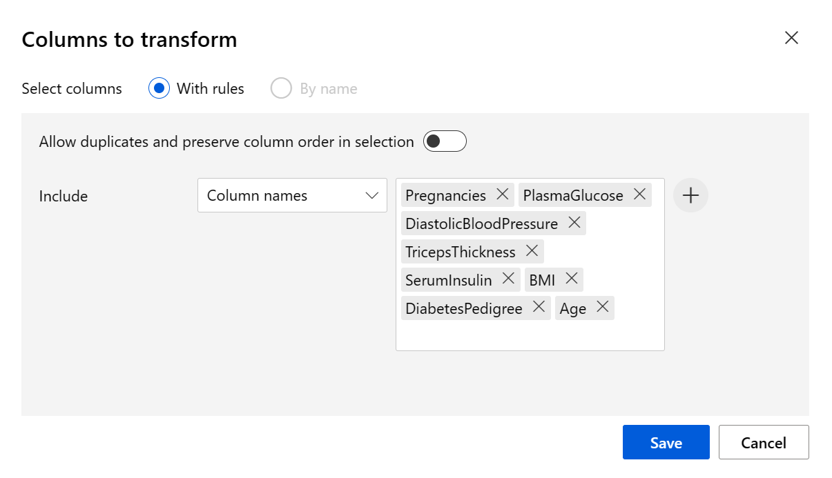
Screenshot of the columns selected for normalization.

Click Save and close the selection box.

The data transformation is normalizing the numeric columns to put them on the same scale, which should help prevent columns with large values from dominating model training. You’d usually apply a whole bunch of pre-processing transformations like this to prepare your data for training, but we’ll keep things simple in this exercise.

Run the pipeline

To apply your data transformations, you need to run the pipeline as an experiment.

Select Configure & Submit at the top of the page to open the Set up pipeline job dialogue.
On the Basics page select Create new and set the name of the experiment to mslearn-diabetes-training then select Next .
On the Inputs & outputs page select Next without making any changes.
On the Runtime settings page an error appears as you don´t have a default compute to run the pipeline. In the Select compute type drop-down select Compute cluster and in the Select Azure ML compute cluster drop-down select your recently created compute cluster.
Select Review + Submit to review the pipeline job and then select Submit to run the training pipeline.
Wait a few minutes for the run to finish. You can check the status of the job by selecting Jobs under the Assets. From there, select the mslearn-diabetes-training experiment and then the Diabetes Training job.

View the transformed data

When the run has completed, the dataset is now prepared for model training.

Right-click (Ctrl+click on a Mac) the Normalize Data module on the canvas, and select Preview data. Select Transformed dataset.
View the data, noting that the numeric columns you selected have been normalized to a common scale.
Close the normalized data result visualization. Return to the previous tab.

After you’ve used data transformations to prepare the data, you can use it to train a machine learning model.

Add training modules

It’s common practice to train the model using a subset of the data, while holding back some data with which to test the trained model. This enables you to compare the labels that the model predicts with the actual known labels in the original dataset.

In this exercise, you’re going to work through steps to extend the Diabetes Training pipeline as shown here:

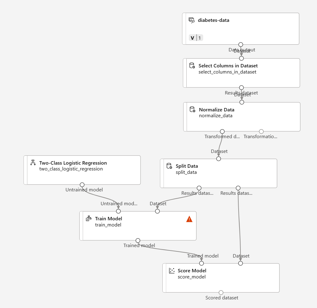
Screenshot of how to split data, then train with logistic regression and score.

Follow the steps below, using the image above for reference as you add and configure the required modules.

Return to the Designer page and select the Diabetes Training pipeline.
In the Asset library pane on the left, in Component, search for and place a Split Data module onto the canvas under the Normalize Data module. Then connect the Transformed Dataset (left) output of the Normalize Data module to the input of the Split Data module.

Tip Use the search bar to quickly locate modules.
Select the Split Data module, and configure its settings as follows:
- Splitting mode: Split Rows
- Fraction of rows in the first output dataset: 0.7
- Randomized split: True
- Random seed: 123
- Stratified split: False
In the Asset library, search for and place a Train Model module to the canvas, under the Split Data module. Then connect the Results dataset1 (left) output of the Split Data module to the Dataset (right) input of the Train Model module.
The model we’re training will predict the Diabetic value, so select the Train Model module and modify its settings to set the Label column to Diabetic.

The Diabetic label the model will predict is a class (0 or 1), so we need to train the model using a classification algorithm. Specifically, there are two possible classes, so we need a binary classification algorithm.
In the Asset library, search for and place a Two-Class Logistic Regression module to the canvas, to the left of the Split Data module and above the Train Model module. Then connect its output to the Untrained model (left) input of the Train Model module.

To test the trained model, we need to use it to score the validation dataset we held back when we split the original data - in other words, predict labels for the features in the validation dataset.
In the Asset library, search for and place a Score Model module to the canvas, below the Train Model module. Then connect the output of the Train Model module to the Trained model (left) input of the Score Model module; and connect the Results dataset2 (right) output of the Split Data module to the Dataset (right) input of the Score Model module.

Run the training pipeline

Now you’re ready to run the training pipeline and train the model.

Select Configure & Submit, and run the pipeline using the existing experiment named mslearn-diabetes-training.
Wait for the experiment run to finish. This may take 5 minutes or more.
Check the status of the job by selecting Jobs under the Assets. From there, select the mslearn-diabetes-training experiment and then select the latest Diabetes Training job.
On the new tab, right-click (Ctrl+click on a Mac) the Score Model module on the canvas, select Preview data and then select Scored dataset to view the results.
Scroll to the right, and note that next to the Diabetic column (which contains the known true values of the label) there is a new column named Scored Labels, which contains the predicted label values, and a Scored Probabilities column containing a probability value between 0 and 1. This indicates the probability of a positive prediction, so probabilities greater than 0.5 result in a predicted label of 1 (diabetic), while probabilities between 0 and 0.5 result in a predicted label of 0 (not diabetic).
Close the Scored_dataset tab.

The model is predicting values for the Diabetic label, but how reliable are its predictions? To assess that, you need to evaluate the model.

The validation data you held back and used to score the model includes the known values for the label. So to validate the model, you can compare the true values for the label to the label values that were predicted when you scored the validation dataset. Based on this comparison, you can calculate various metrics that describe how well the model performs.

Add an Evaluate Model module

Return to Designer and open the Diabetes Training pipeline you created.
In the Asset library, search for and place an Evaluate Model module to the canvas, under the Score Model module, and connect the output of the Score Model module to the Scored dataset (left) input of the Evaluate Model module.
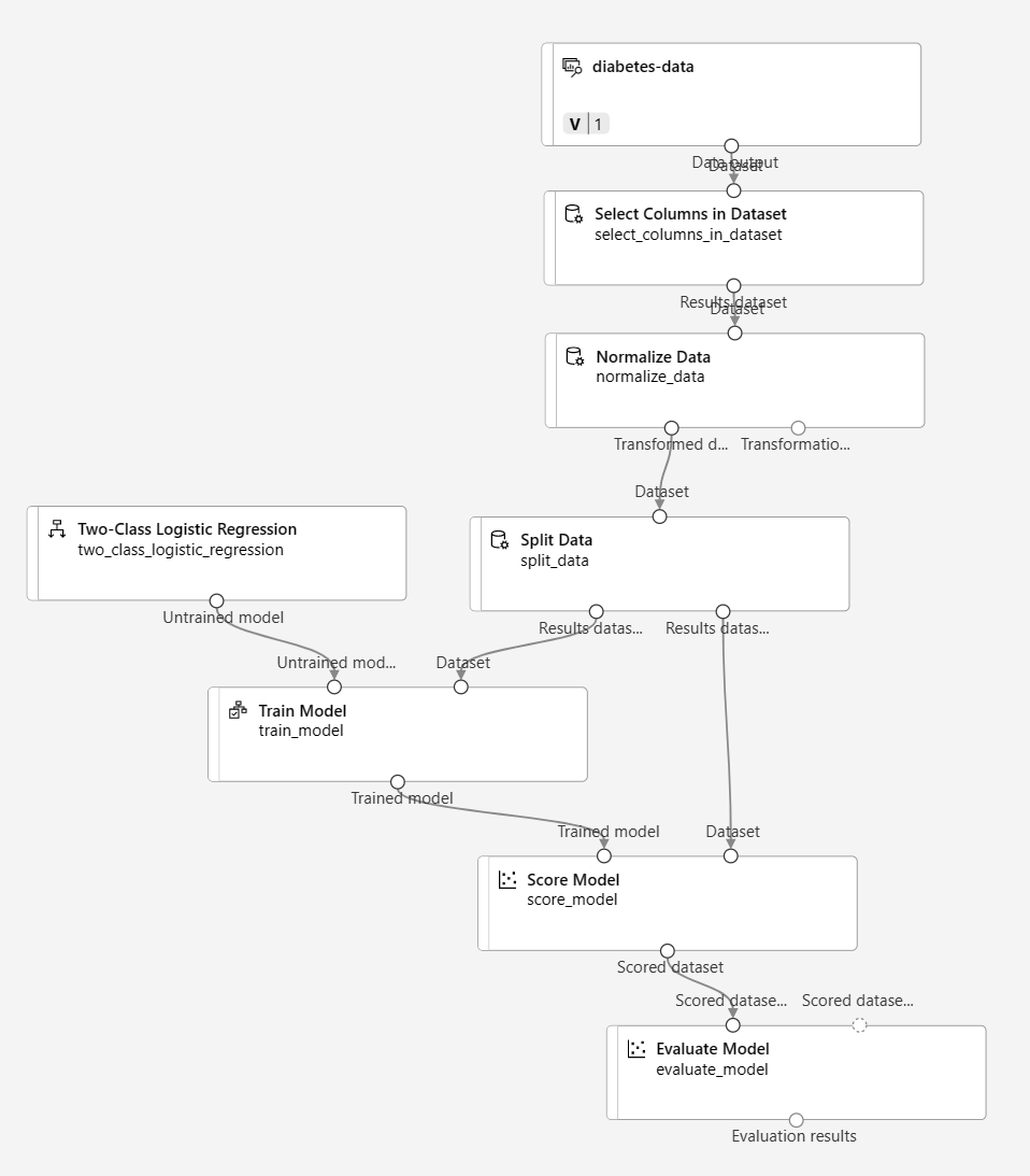
Ensure your pipeline looks like this:
Select Configure & Submit, and run the pipeline using the existing experiment named mslearn-diabetes-training.
Wait for the experiment run to finish.
Check the status of the job by selecting Jobs under the Assets. From there, select the mslearn-diabetes-training experiment and then select the latest Diabetes Training job.
On the new tab, right-click (Ctrl+click on a Mac) the Evaluate Model module on the canvas, select Preview data then select Evaluation results to view the performance metrics. These metrics can help data scientists assess how well the model predicts based on the validation data.
Scroll down to view the confusion matrix for the model. Observe the predicted and actual value counts for each possible class.
Review the metrics to the left of the confusion matrix, which include:
- Accuracy: In other words, what proportion of diabetes predictions did the model get right?
- Precision: In other words, out of all the patients that the model predicted as having diabetes, the percentage of time the model is correct.
- Recall: In other words, out of all the patients who actually have diabetes, how many diabetic cases did the model identify correctly?
- F1 Score
Use the Threshold slider located above the list of metrics. Try moving the threshold slider and observe the effect on the confusion matrix. If you move it all the way to the left (0), the Recall metric becomes 1, and if you move it all the way to the right (1), the Recall metric becomes 0.
Look above the Threshold slider at the ROC curve and AUC metric listed with the other metrics below. To get an idea of how this area represents the performance of the model, imagine a straight diagonal line from the bottom left to the top right of the ROC chart. This represents the expected performance if you just guessed or flipped a coin for each patient - you could expect to get around half of them right, and half of them wrong, so the area under the diagonal line represents an AUC of 0.5. If the AUC for your model is higher than this for a binary classification model, then the model performs better than a random guess.
Close the Evaluation_results tab.

The performance of this model isn’t all that great, partly because we performed only minimal feature engineering and pre-processing. You could try a different classification algorithm, such as Two-Class Decision Forest, and compare the results. You can connect the outputs of the Split Data module to multiple Train Model and Score Model modules, and you can connect a second Score Model module to the Evaluate Model module to see a side-by-side comparison. The point of the exercise is simply to introduce you to classification and the Azure Machine Learning designer interface, not to train a perfect model!

Create an inference pipeline

Locate the menu above the canvas and select Create inference pipeline. You may need to expand your screen to full and click on the three dots icon … on the top right hand corner of the screen in order to find Create inference pipeline in the menu.
In the Create inference pipeline drop-down list, select Real-time inference pipeline. After a few seconds, a new version of your pipeline named Diabetes Training-real time inference will be opened.
Rename the new pipeline to Predict Diabetes, and then review the new pipeline. Some of the transformations and training steps are a part of this pipeline. The trained model will be used to score the new data. The pipeline also contains a web service output to return results.

You’re going to make the following changes to the inference pipeline:
- Add a web service input component for new data to be submitted.
- Replace the diabetes-data dataset with an Enter Data Manually module that doesn’t include the label column (Diabetic).
- Edit the columns selected in the Select Columns in Dataset module.
- Remove the Evaluate Model module.
- Insert an Execute Python Script module before the web service output to return only the patient ID, predicted label value, and probability.
The pipeline does not automatically include a Web Service Input component for models created from custom data sets. Search for a Web Service Input component from the asset library and place it at the top of the pipeline. Connect the output of the Web Service Input component to the Select Columns in Dataset component that is already on the canvas.
The inference pipeline assumes that new data will match the schema of the original training data, so the diabetes-data dataset from the training pipeline is included. However, this input data includes the Diabetic label that the model predicts, which is not included in new patient data for which a diabetes prediction hasn’t yet been made. Delete this module and replace it with an Enter Data Manually module, containing the following CSV data, which includes feature values without labels for three new patient observations:
```
 PatientID,Pregnancies,PlasmaGlucose,DiastolicBloodPressure,TricepsThickness,SerumInsulin,BMI,DiabetesPedigree,Age
 1882185,9,104,51,7,24,27.36983156,1.350472047,43
 1662484,6,73,61,35,24,18.74367404,1.074147566,75
 1228510,4,115,50,29,243,34.69215364,0.741159926,59
```
Connect the new Enter Data Manually module to the same Dataset input of the Select Columns in Dataset module as the Web Service Input.
Edit the Select Columns in Dataset module. Remove Diabetic from the Selected Columns.
The inference pipeline includes the Evaluate Model module, which isn’t useful when predicting from new data, so delete this module.
The output from the Score Model module includes all of the input features and the predicted label and probability score. To limit the output to only the prediction and probability:
- Delete the connection between the Score Model module and the Web Service Output.
- Add an Execute Python Script module, replacing all of the default python script with the following code (which selects only the PatientID, Scored Labels and Scored Probabilities columns and renames them appropriately):
```
 import pandas as pd
    
 def azureml_main(dataframe1 = None, dataframe2 = None):
    
     scored_results = dataframe1[['Scored Labels', 'Scored Probabilities']]
     scored_results.rename(columns={'Scored Labels':'DiabetesPrediction',
                                 'Scored Probabilities':'Probability'},
                         inplace=True)
     return scored_results
```
Connect the output from the Score Model module to the Dataset1 (left-most) input of the Execute Python Script, and connect the Result dataset (left) output of the Execute Python Script module to the Web Service Output.
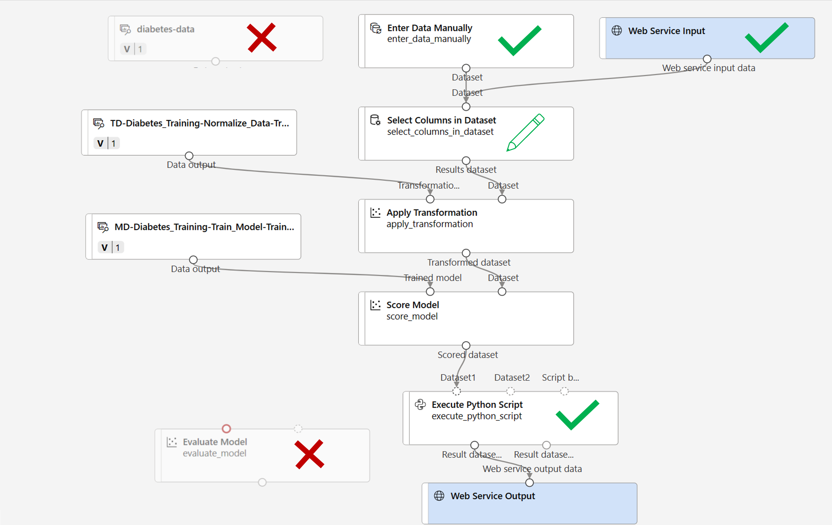
Verify that your pipeline looks similar to the following image:
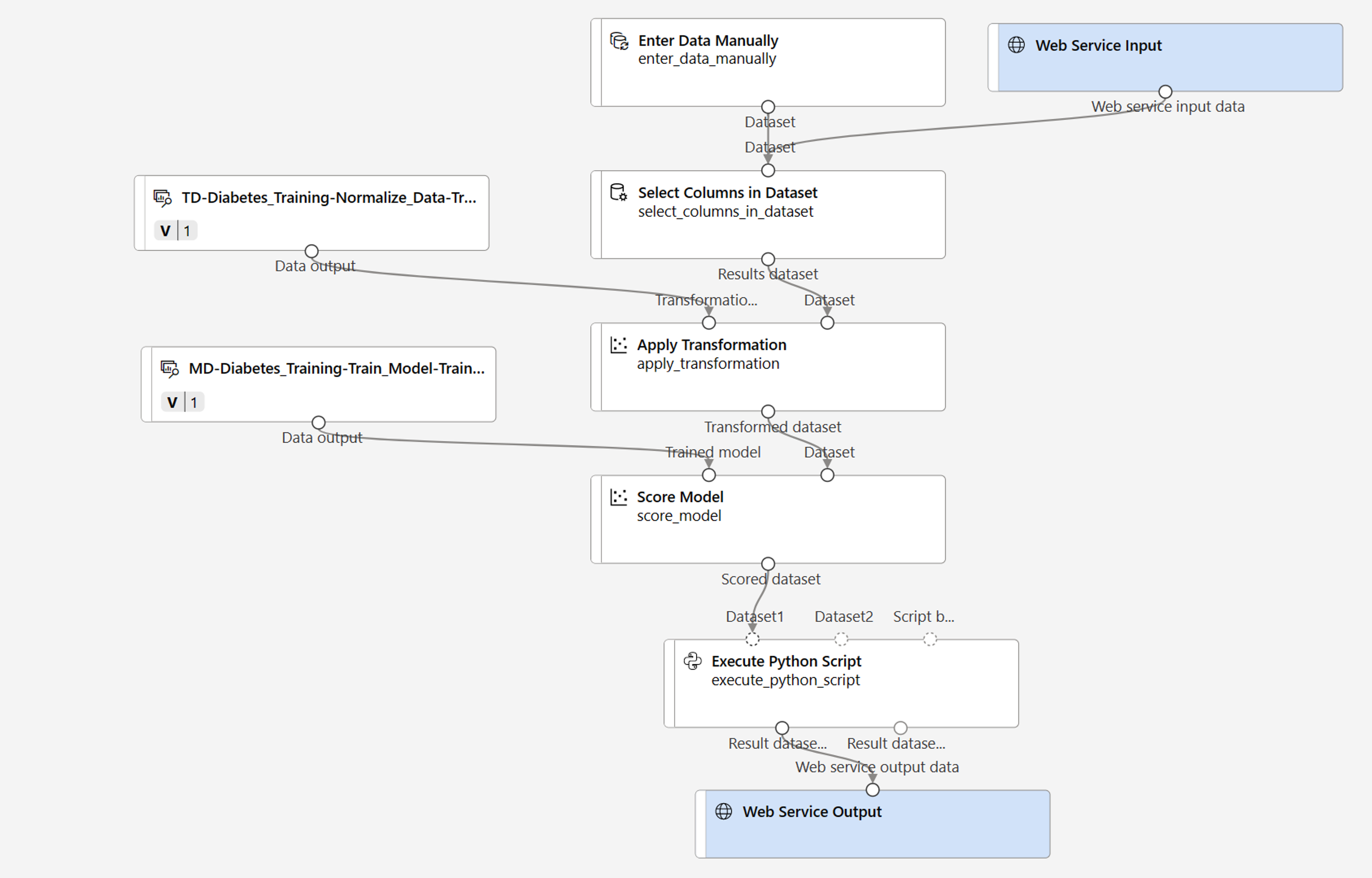
Run the pipeline as a new experiment named mslearn-diabetes-inference on your compute cluster. The experiment may take a while to run.
Return to the Jobs tab. From there, select the mslearn-diabetes-inference experiment and then select the Predict Diabetes job.
When the pipeline has completed, select the Execute Python Script module. Select the Preview data and select Result dataset to see the predicted labels and probabilities for the three patient observations in the input data.

Your inference pipeline predicts whether or not patients are at risk for diabetes based on their features. Now you’re ready to publish the pipeline so that client applications can use it.

After you’ve created and tested an inference pipeline for real-time inferencing, you can publish it as a service for client applications to use.

Note In this exercise, you’ll deploy the web service to an Azure Container Instance (ACI). This type of compute is created dynamically, and is useful for development and testing. For production, you should create an inference cluster, which provide an Azure Kubernetes Service (AKS) cluster that provides better scalability and security.

Deploy a service

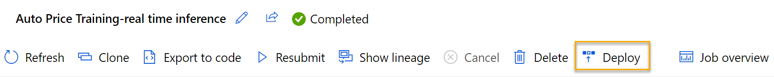
At the top of the Predict Diabetes job window, select Deploy.
In the Set up real-time endpoint select Deploy new real-time endpoint and use the following settings:
- Name: predict-diabetes
- Description: Classify diabetes
- Compute type: Azure Container Instance
Select Deploy and wait for the web service to be deployed - this can take several minutes.

Test the service

On the Endpoints page, open the predict-diabetes real-time endpoint.

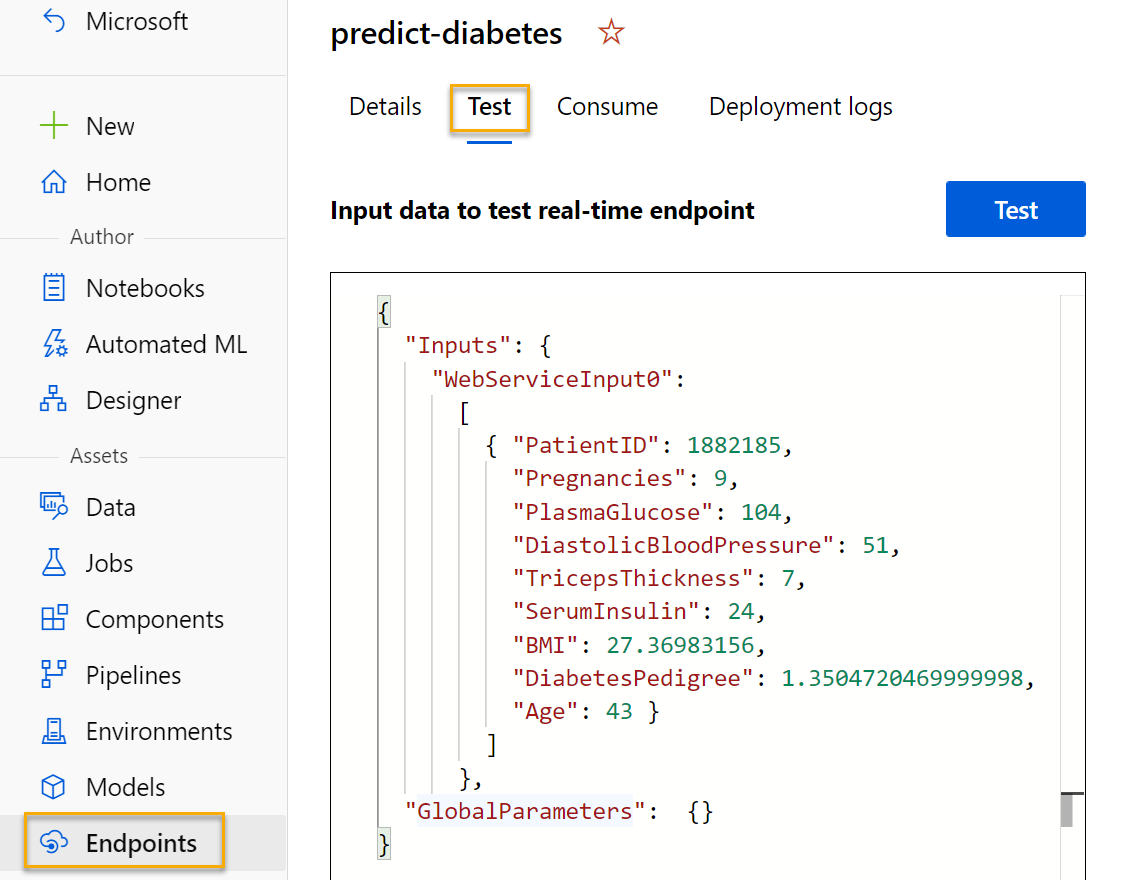
When the predict-diabetes endpoint opens, select the Test tab. We will use it to test our model with new data. Delete the current data under Input data to test real-time endpoint. Copy and paste the below data into the data section:

 {
   "Inputs": {
     "input1":
       [
         { "PatientID": 1882185,
           "Pregnancies": 9,
           "PlasmaGlucose": 104,
           "DiastolicBloodPressure": 51,
           "TricepsThickness": 7,
           "SerumInsulin": 24,
           "BMI": 27.36983156,
           "DiabetesPedigree": 1.3504720469999998,
           "Age": 43 }
         ]
       },
   "GlobalParameters":  {}
 }

Note The JSON above defines features for a patient, and uses the predict-diabetes service you created to predict a diabetes diagnosis.

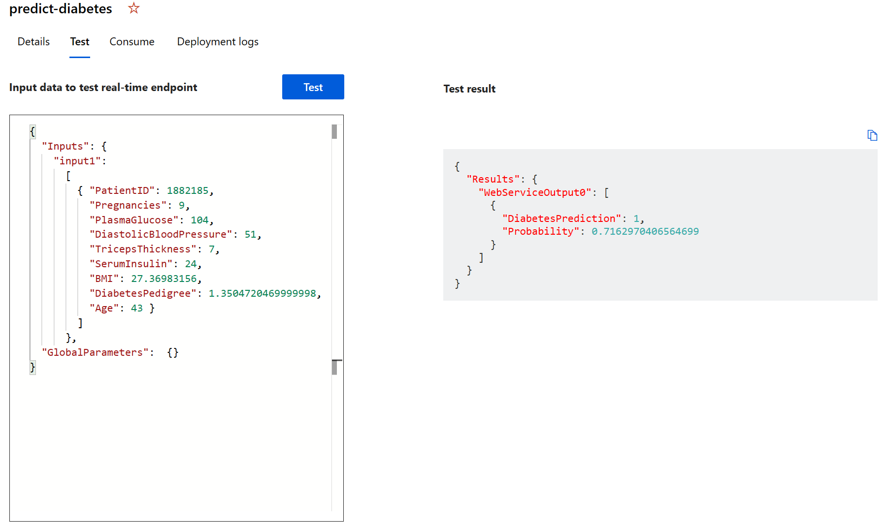
Select Test. On the right hand of the screen, you should see the output ‘DiabetesPrediction’. The output is 1 if the patient is predicted to have diabetes, and 0 if the patient is predicted not to have diabetes.

You have just tested a service that is ready to be connected to a client application using the credentials in the Consume tab. We will end the lab here. You are welcome to continue to experiment with the service you just deployed.

Clean-up

The web service you created is hosted in an Azure Container Instance. If you don’t intend to experiment with it further, you should delete the endpoint to avoid accruing unnecessary Azure usage. You should also delete the compute cluster.

In Azure Machine Learning studio, on the Endpoints tab, select the predict-diabetes endpoint. Then select Delete and confirm that you want to delete the endpoint.
On the Compute page, on the Compute clusters tab, select your compute cluster and then select Delete.

Note Deleting your compute ensures your subscription won’t be charged for compute resources. You will however be charged a small amount for data storage as long as the Azure Machine Learning workspace exists in your subscription. If you have finished exploring Azure Machine Learning, you can delete the Azure Machine Learning workspace and associated resources. However, if you plan to complete any other labs in this series, you will need to recreate it.

To delete your workspace:

In the Azure portal, in the Resource groups page, open the resource group you specified when creating your Azure Machine Learning workspace.

Click Delete resource group, type the resource group name to confirm you want to delete it, and select Delete.